 Matlab
 Simulink
 NS3
NS3 OMNET++
 COOJA
COOJA CONTIKI OS
 NS2
NS2
Using Python for Research is really tuff task for beginners, so it is advisable to get our technical experts help we will help you with all types of coding and simulation results. We are the leading experts who provide customized solution for the scholars. Share us all your research details by mail, we will help you within few minutes with best research guidance.
Python is considered as an extremely efficient programming language for research algorithms, because of its simplicity, wide library assistance, and legibility. Across different fields, various research algorithms can be applied, tested, and examined through the use of Python. In order to utilize Python for several research algorithms such as data analysis, machine learning, and mathematical optimization, we summarize explicit procedures and instances.
- Mathematical Optimization Algorithms
Instance: Linear Programming using PuLP
The process of enhancing a linear objective function based on linear conditions is included in the linear programming.
# Install the PuLP library
!pip install pulp
import pulp
# Create a linear programming problem
lp_problem = pulp.LpProblem(“MaximizeProfit”, pulp.LpMaximize)
# Define decision variables
x = pulp.LpVariable(‘x’, lowBound=0, cat=’Continuous’)
y = pulp.LpVariable(‘y’, lowBound=0, cat=’Continuous’)
# Objective function
lp_problem += 40 * x + 30 * y
# Constraints
lp_problem += 2 * x + y <= 20
lp_problem += 4 * x + 3 * y <= 60
lp_problem += x + 2 * y <= 15
# Solve the problem
lp_problem.solve()
# Print results
print(f”Optimal value for x: {pulp.value(x)}”)
print(f”Optimal value for y: {pulp.value(y)}”)
print(f”Maximum profit: {pulp.value(lp_problem.objective)}”)
- Machine Learning Algorithms
Instance: Applying a Simple Linear Regression with scikit-learn
Among a dependent factor and one or multiple independent factors, the relevant connection can be designed through the utilization of linear regression.
# Install scikit-learn
!pip install scikit-learn
import numpy as np
from sklearn.linear_model import LinearRegression
import matplotlib.pyplot as plt
# Generate some data
np.random.seed(0)
X = 2 * np.random.rand(100, 1)
y = 4 + 3 * X + np.random.randn(100, 1)
# Train the linear regression model
model = LinearRegression()
model.fit(X, y)
# Make predictions
X_new = np.array([[0], [2]])
y_pred = model.predict(X_new)
# Plot the results
plt.scatter(X, y)
plt.plot(X_new, y_pred, color=’red’, linewidth=2)
plt.xlabel(‘X’)
plt.ylabel(‘y’)
plt.title(‘Linear Regression’)
plt.show()
print(f”Intercept: {model.intercept_}”)
print(f”Coefficient: {model.coef_}”)
- Data Analysis Algorithms
Instance: Time Series Analysis using statsmodels
Examining time-related data points is encompassed in the time series analysis.
# Install statsmodels
!pip install statsmodels
import pandas as pd
import statsmodels.api as sm
import matplotlib.pyplot as plt
# Load a time series dataset
data = sm.datasets.co2.load_pandas().data
data = data.fillna(data.bfill())
# Plot the time series data
data.plot(figsize=(10, 6))
plt.title(‘CO2 Levels Over Time’)
plt.show()
# Perform seasonal decomposition
decomposition = sm.tsa.seasonal_decompose(data, model=’additive’)
fig = decomposition.plot()
plt.show()
- Graph Algorithms
Instance: Shortest Path using networkx
For issues relevant to network structures, the graph algorithms are highly suitable.
# Install networkx
!pip install networkx
import networkx as nx
# Create a directed graph
G = nx.DiGraph()
# Add edges with weights
G.add_weighted_edges_from([
(‘A’, ‘B’, 1),
(‘B’, ‘C’, 2),
(‘A’, ‘C’, 2),
(‘C’, ‘D’, 1)
])
# Compute the shortest path
shortest_path = nx.shortest_path(G, source=’A’, target=’D’, weight=’weight’)
path_length = nx.shortest_path_length(G, source=’A’, target=’D’, weight=’weight’)
print(f”Shortest path: {shortest_path}”)
print(f”Path length: {path_length}”)
- Genetic Algorithms
Instance: Resolving an Optimization Problem using DEAP
Through representing the natural selection procedure, the genetic algorithms are employed for various optimization issues.
# Install DEAP
!pip install deap
import random
from deap import base, creator, tools, algorithms
# Define the problem as maximizing the sum of a list
creator.create(“FitnessMax”, base.Fitness, weights=(1.0,))
creator.create(“Individual”, list, fitness=creator.FitnessMax)
toolbox = base.Toolbox()
toolbox.register(“attr_bool”, random.randint, 0, 1)
toolbox.register(“individual”, tools.initRepeat, creator.Individual, toolbox.attr_bool, n=100)
toolbox.register(“population”, tools.initRepeat, list, toolbox.individual)
def evalOneMax(individual):
return sum(individual),
toolbox.register(“evaluate”, evalOneMax)
toolbox.register(“mate”, tools.cxTwoPoint)
toolbox.register(“mutate”, tools.mutFlipBit, indpb=0.05)
toolbox.register(“select”, tools.selTournament, tournsize=3)
population = toolbox.population(n=300)
ngen, cxpb, mutpb = 40, 0.5, 0.2
result = algorithms.eaSimple(population, toolbox, cxpb, mutpb, ngen, verbose=False)
# Extracting the best individual
best_individual = tools.selBest(population, k=1)[0]
print(f”Best individual: {best_individual}”)
print(f”Fitness: {best_individual.fitness.values[0]}”)
Python research Thesis services
In various research departments, Python is employed in an extensive manner for several purposes. To apply Python in diverse research departments, we suggest a clear outline which encompasses various project plans and explicit instances:
- Computer Science Department
Project Plans:
- Machine Learning Model Development
- Cybersecurity Simulations
- Algorithm Analysis and Visualization
- Big Data Analytics
- Natural Language Processing
Instance: Machine Learning Model Development
# Install scikit-learn
!pip install scikit-learn
from sklearn.datasets import load_iris
from sklearn.model_selection import train_test_split
from sklearn.ensemble import RandomForestClassifier
from sklearn.metrics import accuracy_score
# Load dataset
data = load_iris()
X = data.data
y = data.target
# Split the dataset
X_train, X_test, y_train, y_test = train_test_split(X, y, test_size=0.3, random_state=42)
# Train a RandomForest model
model = RandomForestClassifier(n_estimators=100)
model.fit(X_train, y_train)
# Make predictions
y_pred = model.predict(X_test)
# Evaluate the model
accuracy = accuracy_score(y_test, y_pred)
print(f”Accuracy: {accuracy}”)
- Physics Department
Project Plans:
- Quantum Computing Simulations
- Thermodynamics Simulations
- Astrophysics Data Analysis
- Simulating Physical Systems
- Particle Physics Simulations
Instance: Simulating a Pendulum
import numpy as np
import matplotlib.pyplot as plt
# Parameters
g = 9.81 # Gravity
L = 1.0 # Length of the pendulum
theta0 = np.pi / 4 # Initial angle
omega0 = 0.0 # Initial angular velocity
t_max = 10.0 # Simulation time
dt = 0.01 # Time step
# Time array
t = np.arange(0, t_max, dt)
# Arrays to store the angle and angular velocity
theta = np.zeros_like(t)
omega = np.zeros_like(t)
# Initial conditions
theta[0] = theta0
omega[0] = omega0
# Euler’s method
for i in range(1, len(t)):
omega[i] = omega[i-1] – (g / L) * np.sin(theta[i-1]) * dt
theta[i] = theta[i-1] + omega[i] * dt
# Plot the results
plt.figure(figsize=(10, 5))
plt.plot(t, theta, label=’Angle (theta)’)
plt.plot(t, omega, label=’Angular Velocity (omega)’)
plt.xlabel(‘Time (s)’)
plt.ylabel(‘Value’)
plt.legend()
plt.title(‘Pendulum Simulation’)
plt.show()
- Biology Department
Project Plans:
- Bioinformatics Algorithms
- Genomic Data Analysis
- Ecological Modeling
- Simulating Biological Processes
- Epidemiological Simulations
Instance: Population Growth Simulation
import numpy as np
import matplotlib.pyplot as plt
# Parameters
r = 0.1 # Growth rate
K = 1000 # Carrying capacity
N0 = 10 # Initial population
t_max = 100 # Time period
dt = 1 # Time step
# Time array
t = np.arange(0, t_max, dt)
# Population array
N = np.zeros_like(t)
N[0] = N0
# Logistic growth model
for i in range(1, len(t)):
N[i] = N[i-1] + r * N[i-1] * (1 – N[i-1] / K) * dt
# Plot the results
plt.figure(figsize=(10, 5))
plt.plot(t, N, label=’Population (N)’)
plt.xlabel(‘Time’)
plt.ylabel(‘Population’)
plt.legend()
plt.title(‘Population Growth Simulation’)
plt.show()
- Chemistry Department
Project Plans:
- Chemical Kinetics Modeling
- Spectroscopy Data Analysis
- Molecular Dynamics Simulations
- Drug Discovery Simulations
- Quantum Chemistry Calculations
Instance: Reaction Kinetics Simulation
import numpy as np
import matplotlib.pyplot as plt
# Parameters
k = 0.01 # Reaction rate constant
A0 = 1.0 # Initial concentration of A
B0 = 0.0 # Initial concentration of B
t_max = 100 # Time period
dt = 1 # Time step
# Time array
t = np.arange(0, t_max, dt)
# Concentration arrays
A = np.zeros_like(t)
B = np.zeros_like(t)
A[0] = A0
B[0] = B0
# Reaction kinetics model
for i in range(1, len(t)):
A[i] = A[i-1] – k * A[i-1] * dt
B[i] = B[i-1] + k * A[i-1] * dt
# Plot the results
plt.figure(figsize=(10, 5))
plt.plot(t, A, label=’Concentration of A’)
plt.plot(t, B, label=’Concentration of B’)
plt.xlabel(‘Time’)
plt.ylabel(‘Concentration’)
plt.legend()
plt.title(‘Reaction Kinetics Simulation’)
plt.show()
- Economics Department
Project Plans:
- Financial Market Analysis
- Macroeconomic Data Analysis
- Game Theory Simulations
- Economic Modeling and Simulation
- Behavioral Economics Experiments
Instance: Simulating Market Demand and Supply
import numpy as np
import matplotlib.pyplot as plt
# Parameters
P = np.linspace(0.01, 10, 100) # Price range
a = 50 # Demand intercept
b = 2 # Demand slope
c = 10 # Supply intercept
d = 1.5 # Supply slope
# Demand and supply functions
D = a – b * P # Demand
S = c + d * P # Supply
# Find equilibrium price and quantity
P_eq = (a – c) / (b + d)
Q_eq = a – b * P_eq
# Plot the results
plt.figure(figsize=(10, 5))
plt.plot(P, D, label=’Demand’)
plt.plot(P, S, label=’Supply’)
plt.axvline(x=P_eq, color=’r’, linestyle=’–‘, label=f’Equilibrium Price: {P_eq:.2f}’)
plt.axhline(y=Q_eq, color=’g’, linestyle=’–‘, label=f’Equilibrium Quantity: {Q_eq:.2f}’)
plt.xlabel(‘Price’)
plt.ylabel(‘Quantity’)
plt.legend()
plt.title(‘Market Demand and Supply Simulation’)
plt.show()
- Psychology Department
Project Plans:
- Psychometric Test Simulations
- Cognitive Model Simulations
- Simulating Decision-Making Processes
- Behavioral Data Analysis
- Neuroimaging Data Analysis
Instance: Reaction Time Experiment Simulation
import numpy as np
import matplotlib.pyplot as plt
# Parameters
n_trials = 100
mean_reaction_time = 250 # Mean reaction time in milliseconds
std_reaction_time = 50 # Standard deviation in milliseconds
# Simulate reaction times
reaction_times = np.random.normal(mean_reaction_time, std_reaction_time, n_trials)
# Plot the results
plt.figure(figsize=(10, 5))
plt.hist(reaction_times, bins=15, edgecolor=’black’)
plt.xlabel(‘Reaction Time (ms)’)
plt.ylabel(‘Frequency’)
plt.title(‘Reaction Time Experiment Simulation’)
plt.show()
print(f”Mean Reaction Time: {np.mean(reaction_times):.2f} ms”)
print(f”Standard Deviation: {np.std(reaction_times):.2f} ms”)
- Environmental Science Department
Project Plans:
- Ecosystem Simulation
- Renewable Energy Simulation
- Climate Change Modeling
- Water Resource Management
- Pollution Spread Simulation
Instance: CO2 Emissions Reduction Simulation
import numpy as np
import matplotlib.pyplot as plt
# Parameters
years = np.arange(2020, 2051)
emissions_2020 = 10 # Emissions in 2020 (GtCO2)
reduction_rate = 0.03 # Annual reduction rate
# Simulate emissions over time
emissions = emissions_2020 * (1 – reduction_rate) ** (years – 2020)
# Plot the results
plt.figure(figsize=(10, 5))
plt.plot(years, emissions, label=’CO2 Emissions’)
plt.xlabel(‘Year’)
plt.ylabel(‘Emissions (GtCO2)’)
plt.legend()
plt.title(‘CO2 Emissions Reduction Simulation’)
plt.show()
As a means to employ Python for various research algorithms, some instances and procedures are summarized by us. For assisting you to utilize Python in diverse research departments, we offered an outline, including various instances and project plans which are intriguing as well as significant.
Subscribe Our Youtube Channel
You can Watch all Subjects Matlab & Simulink latest Innovative Project Results

Our services
We want to support Uncompromise Matlab service for all your Requirements Our Reseachers and Technical team keep update the technology for all subjects ,We assure We Meet out Your Needs.
Our Services
- Matlab Research Paper Help
- Matlab assignment help
- Matlab Project Help
- Matlab Homework Help
- Simulink assignment help
- Simulink Project Help
- Simulink Homework Help
- Matlab Research Paper Help
- NS3 Research Paper Help
- Omnet++ Research Paper Help
Our Benefits
- Customised Matlab Assignments
- Global Assignment Knowledge
- Best Assignment Writers
- Certified Matlab Trainers
- Experienced Matlab Developers
- Over 400k+ Satisfied Students
- Ontime support
- Best Price Guarantee
- Plagiarism Free Work
- Correct Citations
Expert Matlab services just 1-click

Delivery Materials
Unlimited support we offer you
For better understanding purpose we provide following Materials for all Kind of Research & Assignment & Homework service.
 Programs
 Designs
 Simulations
 Results
 Graphs
 Result snapshot
 Video Tutorial
 Instructions Profile
  Sofware Install Guide
 Execution Guidance
  Explanations
 Implement Plan
Matlab Projects
Matlab projects innovators has laid our steps in all dimension related to math works.Our concern support matlab projects for more than 10 years.Many Research scholars are benefited by our matlab projects service.We are trusted institution who supplies matlab projects for many universities and colleges.
Reasons to choose Matlab Projects .org???
Our Service are widely utilized by Research centers.More than 5000+ Projects & Thesis has been provided by us to Students & Research Scholars. All current mathworks software versions are being updated by us.
Our concern has provided the required solution for all the above mention technical problems required by clients with best Customer Support.
- Novel Idea
- Ontime Delivery
- Best Prices
- Unique Work
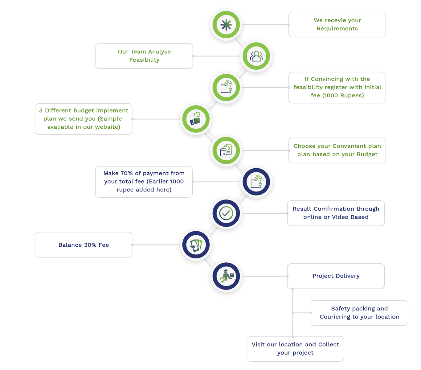
Simulation Projects Workflow
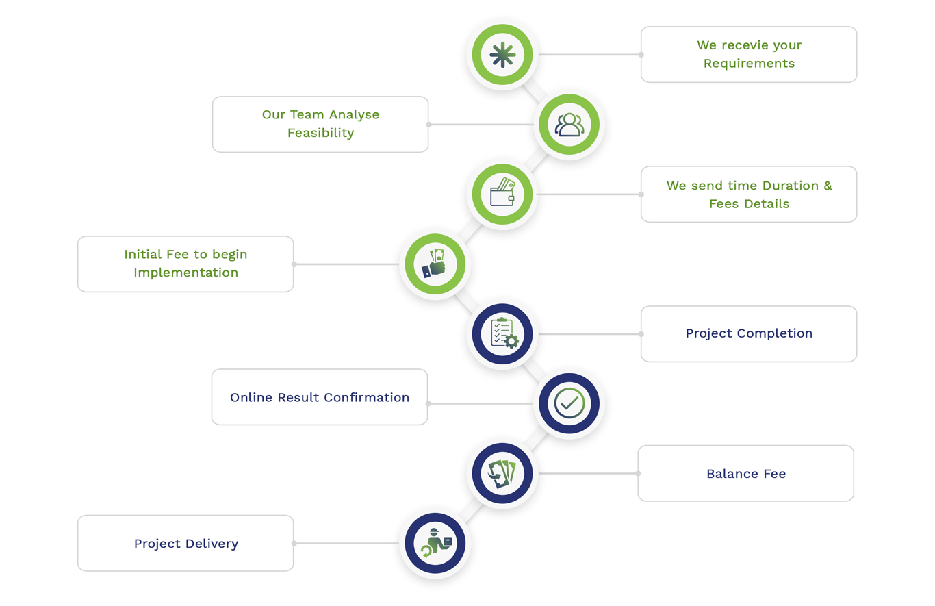
Embedded Projects Workflow