 Matlab
 Simulink
 NS3
NS3 OMNET++
 COOJA
COOJA CONTIKI OS
 NS2
NS2
Python Numerical Simulation assistance are provided by us drop a message to matlabprojects.org we will help you with results. Explore the utilization of Python for numerical analysis we guide you with our comprehensive tools and libraries. Reach out to us for professional support and to achieve the best outcomes. Numerical simulation is examined as both an intricate and significant process that must be carried out by following specific guidelines. To conduct this process efficiently, we suggest a few prevalent algorithms and parameters, along with brief outlines:
- Finite Difference Method (FDM)
- Algorithm: Through estimating derivatives with finite differences, the differential equations can be resolved by this method.
- Relevant Parameters:
- Grid spacing (Δx, Δt)
- Initial conditions
- Boundary conditions
- Time step size
- Finite Element Method (FEM)
- Algorithm: For complicated boundary and initial value issues, this algorithm is widely employed. It assists to segment the field into various components.
- Relevant Parameters:
- Element shape
- Mesh size
- Initial conditions
- Boundary conditions
- Material properties
- Monte Carlo Simulation
- Algorithm: This method is mostly utilized for probabilistic and statistical issues. In order to acquire numerical outcomes, it employs random sampling.
- Relevant Parameters:
- Number of simulations
- Probability distributions
- Random seed
- Sample size
- Runge-Kutta Methods
- Algorithm: To resolve ODEs (ordinary differential equations) with more preciseness, the Runge-Kutta methods are highly suitable.
- Relevant Parameters:
- Initial conditions
- Order of the method (for instance: 4th order Runge-Kutta)
- Time step size
- Particle Swarm Optimization (PSO)
- Algorithm: PSO is referred to as an optimization approach, which is specifically derived from the fish or birds’ social activity.
- Relevant Parameters:
- Number of particles
- Maximum velocity
- Cognitive and social coefficients
- Inertia weight
- Genetic Algorithms
- Algorithm: It is an optimization method, which is facilitated by natural selection.
- Relevant Parameters:
- Number of generations
- Population size
- Mutation rate
- Crossover rate
- Gradient Descent
- Algorithm: For identifying the least of a function, this optimization approach is appropriate.
- Relevant Parameters:
- Convergence criteria
- Batch size (for stochastic gradient descent)
- Learning rate
- Number of iterations
Python Libraries and Tools
- NumPy: It is highly ideal for array management and numerical operations.
- SciPy: Scientific calculation and incorporation can be facilitated by SciPy.
- Matplotlib: This tool is more suitable for visualization and plotting.
- SymPy: Make use of SymPy for symbolic mathematics.
- Pyomo: It is generally utilized for optimization issues.
- SimPy: For discrete-event simulation, it is more useful.
Python numerical simulation projects
The process of resolving mathematical models of physical events with computational approaches is included in the numerical simulation. For numerical simulations, Python is an appropriate and robust tool because of having a wide range of libraries like Matplotlib, SciPy, and NumPy. By encompassing various topics, we list out numerous Python project plans related to numerical simulation:
- Heat Equation Simulation
- Explanation: To analyze heat diffusion periodically, the 1D or 2D heat equation has to be resolved with finite difference methods.
- Major Characteristics: Stability exploration, explicit and implicit techniques, and visualization of temperature diffusion.
- Projectile Motion Simulation
- Explanation: In the impact of air resistance and gravity, the movement of a projectile must be simulated.
- Major Characteristics: Impact of air resistance, equations of motion, and trajectory plotting.
- Fluid Flow in a Pipe
- Explanation: Across a pipe, the laminar and turbulent fluid flow should be simulated. For that, we utilize the Navier-Stokes equations.
- Major Characteristics: Pressure loss analysis, velocity profiles, and Reynolds number estimation.
- Pendulum Dynamics
- Explanation: By means of ordinary differential equations (ODEs), the movement of a double and simple pendulum has to be simulated.
- Major Characteristics: Chaotic activity in double pendulums, phase space plots, and nonlinear dynamics.
- Spring-Mass-Damper System
- Explanation: The motions of a spring-mass-damper framework must be designed and simulated.
- Major Characteristics: Resonance exploration, forced vibrations, and damped and undamped oscillations.
- Population Growth Models
- Explanation: Various population growth models have to be applied and simulated. It could include logistic growth, exponential growth, and predator-prey models.
- Major Characteristics: Long-term activity, stability exploration, and differential equations.
- Traffic Flow Simulation
- Explanation: Make use of the cell transmission model or other major traffic flow models to simulate the flow of traffic on a highway.
- Major Characteristics: Congestion exploration, flow and speed connections, and traffic load.
- Wave Equation Simulation
- Explanation: To simulate wave distribution, we plan to resolve the 1D or 2D wave equation.
- Major Characteristics: Visualization of wave movement, finite difference methods, and reflection and distribution at boundaries.
- Epidemic Spread Modeling
- Explanation: By utilizing compartmental models such as SEIR or SIR, the distribution of an infectious disease should be simulated.
- Major Characteristics: Differential equations, intervention policies, recovery rates, and contact rates.
- Orbital Mechanics Simulation
- Explanation: Through Newton’s law of gravitation, the paths of satellites or planets have to be simulated.
- Major Characteristics: Trajectory plotting, Kepler’s laws, n-body problem, and two-body problem.
Instance: Heat Equation Simulation
For resolving the 1D heat equation, we offer an instance, which employs the explicit finite difference method.
Step 1: Import Required Libraries
import numpy as np
import matplotlib.pyplot as plt
Step 2: Specify the Parameters and Initial Conditions
# Parameters
L = 1.0 # Length of the rod
T = 0.5 # Total time
nx = 50 # Number of spatial points
nt = 1000 # Number of time steps
alpha = 0.01 # Thermal diffusivity
# Discretization
dx = L / (nx – 1)
dt = T / nt
# Stability condition
if dt > dx**2 / (2 * alpha):
raise ValueError(“Stability condition violated: dt must be less than dx^2 / (2 * alpha)”)
# Initial condition: u(x,0) = sin(pi * x)
x = np.linspace(0, L, nx)
u = np.sin(np.pi * x)
# Boundary conditions: u(0,t) = u(L,t) = 0
u[0] = u[-1] = 0
Step 3: Time-Stepping Loop
# Time-stepping loop
u_new = np.zeros(nx)
for n in range(nt):
for i in range(1, nx-1):
u_new[i] = u[i] + alpha * dt / dx**2 * (u[i+1] – 2*u[i] + u[i-1])
u = u_new.copy()
Step 4: Plot the Outcomes
plt.plot(x, u, label=’t = 0.5′)
plt.xlabel(‘x’)
plt.ylabel(‘Temperature’)
plt.title(‘1D Heat Equation’)
plt.legend()
plt.show()
A simple simulation of the 1D heat equation is depicted in the above instance. It indicates the preliminary temperature distribution as u(x,0)=sin(πx)u(x,0) = \sin(\pi x)u(x,0)=sin(πx). On the basis of the heat equation, the temperature emerges periodically.
Instance: Projectile Motion Simulation
In order to simulate projectile motion using air resistance, an explicit instance is provided by us.
Step 1: Import Essential Libraries
import numpy as np
import matplotlib.pyplot as plt
Step 2: Specify the Parameters and Initial Conditions
# Parameters
g = 9.81 # Acceleration due to gravity (m/s^2)
m = 0.145 # Mass of the projectile (kg)
C_d = 0.47 # Drag coefficient
rho = 1.225 # Air density (kg/m^3)
A = 0.0042 # Cross-sectional area of the projectile (m^2)
v0 = 30 # Initial velocity (m/s)
theta = 45 # Launch angle (degrees)
# Initial conditions
v0_x = v0 * np.cos(np.radians(theta))
v0_y = v0 * np.sin(np.radians(theta))
# Time settings
dt = 0.01 # Time step (s)
t_max = 5 # Maximum simulation time (s)
Step 3: Specify the Equations of Motion
# Equations of motion with air resistance
def equations_of_motion(v, t):
v_x, v_y = v
speed = np.sqrt(v_x**2 + v_y**2)
F_d = 0.5 * C_d * rho * A * speed**2
F_d_x = F_d * (v_x / speed)
F_d_y = F_d * (v_y / speed)
dv_xdt = – (F_d_x / m)
dv_ydt = – g – (F_d_y / m)
return np.array([dv_xdt, dv_ydt])
Step 4: Time-Stepping Loop
# Time-stepping loop
t = np.arange(0, t_max, dt)
v = np.array([v0_x, v0_y])
positions = []
for ti in t:
positions.append(v * ti)
v = v + equations_of_motion(v, ti) * dt
positions = np.array(positions)
x = positions[:, 0]
y = positions[:, 1]
Step 5: Plot the Outcomes
plt.plot(x, y, label=’Projectile Path’)
plt.xlabel(‘x (m)’)
plt.ylabel(‘y (m)’)
plt.title(‘Projectile Motion with Air Resistance’)
plt.legend()
plt.grid(True)
plt.show()
Across the impact of air resistance and gravity, we simulate the movement of a projectile in this instance. The drag force has to be explained in the equations of motion. It is important to plot the path of the projectile.
Expanding the Simulation
Focus on the below specified improvements to expand these instances:
- Higher Dimensions: The simulations have to be expanded to 3D.
- Variable Properties: It is approachable to consider variable air density, thermal diffusivity, and others.
- Advanced Solvers: For ODEs, innovative numerical techniques such as Runge-Kutta must be utilized.
- Interactive Visualization: By employing libraries such as Dash or Plotly, we have to develop communicative visualizations.
- Optimization: In order to acquire anticipated results, identify the optimal parameters by applying optimization methods.
For performing numerical simulations in an efficient manner, various significant algorithms and parameters are recommended by us. Relevant to numerical simulations, we proposed several Python project plans, along with concise explanations, major characteristics, and explicit instances.
Subscribe Our Youtube Channel
You can Watch all Subjects Matlab & Simulink latest Innovative Project Results

Our services
We want to support Uncompromise Matlab service for all your Requirements Our Reseachers and Technical team keep update the technology for all subjects ,We assure We Meet out Your Needs.
Our Services
- Matlab Research Paper Help
- Matlab assignment help
- Matlab Project Help
- Matlab Homework Help
- Simulink assignment help
- Simulink Project Help
- Simulink Homework Help
- Matlab Research Paper Help
- NS3 Research Paper Help
- Omnet++ Research Paper Help
Our Benefits
- Customised Matlab Assignments
- Global Assignment Knowledge
- Best Assignment Writers
- Certified Matlab Trainers
- Experienced Matlab Developers
- Over 400k+ Satisfied Students
- Ontime support
- Best Price Guarantee
- Plagiarism Free Work
- Correct Citations
Expert Matlab services just 1-click

Delivery Materials
Unlimited support we offer you
For better understanding purpose we provide following Materials for all Kind of Research & Assignment & Homework service.
 Programs
 Designs
 Simulations
 Results
 Graphs
 Result snapshot
 Video Tutorial
 Instructions Profile
  Sofware Install Guide
 Execution Guidance
  Explanations
 Implement Plan
Matlab Projects
Matlab projects innovators has laid our steps in all dimension related to math works.Our concern support matlab projects for more than 10 years.Many Research scholars are benefited by our matlab projects service.We are trusted institution who supplies matlab projects for many universities and colleges.
Reasons to choose Matlab Projects .org???
Our Service are widely utilized by Research centers.More than 5000+ Projects & Thesis has been provided by us to Students & Research Scholars. All current mathworks software versions are being updated by us.
Our concern has provided the required solution for all the above mention technical problems required by clients with best Customer Support.
- Novel Idea
- Ontime Delivery
- Best Prices
- Unique Work
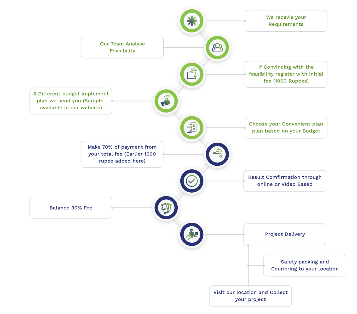
Simulation Projects Workflow

Embedded Projects Workflow