 Matlab
 Simulink
 NS3
NS3 OMNET++
 COOJA
COOJA CONTIKI OS
 NS2
NS2
Python Mechanical Simulation is employed in an extensive manner because of its simple utilization. For numerical computation and visualization, it offers various robust libraries. Here are several project concepts and illustrations for mechanical simulations utilizing Python. If you require assistance with Python simulations, your search ends here! At matlabprojects.org, our specialists provide outstanding support for simulations, catering to all proficiency levels. Please share your project specifications with us. By considering mechanical simulations with Python, we recommend a few interesting project plans and instances:
- Finite Element Analysis (FEA)
- Explanation: In mechanical elements, resolve various structural issues like disfiguration, strain, and stress by applying FEA techniques.
- Major Characteristics: Element rigidity matrix computation, mesh generation, visualization of outcomes, and boundary constraints.
- Computational Fluid Dynamics (CFD)
- Explanation: By means of CFD methods, we simulate the flow of fluids across objects.
- Major Characteristics: Flow visualization, discretization techniques (finite volume, finite difference), and Navier-Stokes equations.
- Dynamic Simulation of Mechanisms
- Explanation: The movement of mechanical systems and connections has to be simulated.
- Major Characteristics: Animation of the system, equations of motion, and kinematic and dynamic analysis.
- Thermal Analysis
- Explanation: Specifically in mechanical frameworks, analyze heat transmission by carrying out the thermal analysis process.
- Major Characteristics: Temperature diffusion visualization, steady-state and transient exploration, and conduction, convection, and radiation models.
- Vibration Analysis
- Explanation: Focus on mechanical frameworks and examine their vibration features.
- Major Characteristics: Damping impacts, reaction to external effects, mode structures, and natural frequencies.
- Material Property Simulation
- Explanation: Across various loading states, we consider the mechanical activity of materials and simulate it.
- Major Characteristics: Fracture method, plasticity models, and stress-strain curves.
Sample Project: Finite Element Analysis of a 2D Truss
In order to conduct a basic 2D truss finite element analysis with Python, an explicit instance is offered by us:
Step 1: Import Required Libraries
import numpy as np
import matplotlib.pyplot as plt
Step 2: Specify the Truss Structure
# Node coordinates (x, y)
nodes = np.array([[0, 0], [1, 0], [1, 1], [2, 1], [2, 0], [3, 0]])
# Element connectivity (start node, end node)
elements = np.array([[0, 1], [1, 2], [1, 4], [2, 3], [2, 4], [3, 4], [4, 5]])
# Element properties (Young’s modulus, area)
E = 210e9 # Young’s modulus in Pascals
A = 1e-4 # Cross-sectional area in square meters
Step 3: Define Functions for FEA
def length_and_cosines(node1, node2):
delta = node2 – node1
L = np.linalg.norm(delta)
cos = delta[0] / L
sin = delta[1] / L
return L, cos, sin
def element_stiffness_matrix(L, cos, sin, E, A):
k = (E * A / L) * np.array([[cos**2, cos*sin, -cos**2, -cos*sin],
[cos*sin, sin**2, -cos*sin, -sin**2],
[-cos**2, -cos*sin, cos**2, cos*sin],
[-cos*sin, -sin**2, cos*sin, sin**2]])
return k
Step 4: Set the Global Stiffness Matrix
# Number of nodes and degrees of freedom (DOF)
num_nodes = nodes.shape[0]
dof = 2 * num_nodes
# Initialize global stiffness matrix
K = np.zeros((dof, dof))
# Assemble global stiffness matrix
for element in elements:
node1, node2 = element
L, cos, sin = length_and_cosines(nodes[node1], nodes[node2])
k = element_stiffness_matrix(L, cos, sin, E, A)
dof_indices = np.array([2*node1, 2*node1+1, 2*node2, 2*node2+1])
for i in range(4):
for j in range(4):
K[dof_indices[i], dof_indices[j]] += k[i, j]
Step 5: Implement Boundary Conditions and Solve
# Boundary conditions (fixed nodes)
fixed_nodes = [0, 5]
free_dof = np.array([i for i in range(dof) if i//2 not in fixed_nodes])
# Load vector (applied loads)
F = np.zeros(dof)
F[3] = -1000 # Apply a downward force of 1000 N at node 2
# Solve for displacements
K_ff = K[np.ix_(free_dof, free_dof)]
F_f = F[free_dof]
U_f = np.linalg.solve(K_ff, F_f)
# Full displacement vector
U = np.zeros(dof)
U[free_dof] = U_f
Step 6: Post-Processing and Visualization
# Extract displacements
displacements = U.reshape(num_nodes, 2)
# Deformed shape
scale_factor = 1e3 # Scale factor for visualization
deformed_nodes = nodes + scale_factor * displacements
# Plot original and deformed truss
plt.figure()
for element in elements:
node1, node2 = element
plt.plot(nodes[[node1, node2], 0], nodes[[node1, node2], 1], ‘bo-‘)
plt.plot(deformed_nodes[[node1, node2], 0], deformed_nodes[[node1, node2], 1], ‘ro–‘)
plt.xlabel(‘X Coordinate (m)’)
plt.ylabel(‘Y Coordinate (m)’)
plt.title(‘Original and Deformed Truss’)
plt.legend([‘Original’, ‘Deformed’])
plt.grid(True)
plt.axis(‘equal’)
plt.show()
Python Mechanical Simulation Projects
Relevant to mechanical simulations, several compelling projects have evolved in a gradual manner. Along with significant characteristics, we suggest various major projects regarding mechanical simulations. To offer an explicit interpretation of possible applications and range, every project encompasses concise outlines.
- Finite Element Analysis (FEA) of a Truss Structure
- Outline: In a 2D or 3D truss framework, examine distortion, strain, and stress through the utilization of FEA.
- Significant Characteristics: Boundary constraints, rigidity matrix computation, mesh generation, and outcome visualization.
- Computational Fluid Dynamics (CFD) Simulation of Airflow
- Outline: With CFD methods, the airflow across objects has to be simulated.
- Significant Characteristics: Discretization approaches (finite volume, finite difference), visualization of flow, and Navier-Stokes equations.
- Dynamic Simulation of a Four-Bar Linkage
- Outline: Consider a four-bar linkage system and simulate its movement.
- Significant Characteristics: Equations of motion, kinematic and dynamic analysis, and animation of the system.
- Thermal Analysis of a Heat Sink
- Outline: In a heat sink, we analyze heat transmission by conducting the thermal analysis process.
- Significant Characteristics: Temperature diffusion visualization, conduction, convection, and radiation models, and steady-state and transient exploration.
- Vibration Analysis of a Cantilever Beam
- Outline: Our project concentrates on a cantilever beam and examines its vibration features.
- Significant Characteristics: Mode structures, damping impacts, reaction to external effects, and natural frequencies.
- Stress Analysis of a Pressure Vessel
- Outline: In internal pressure, focus on identifying the stress distribution. For that, stress analysis must be carried out on a pressure vessel.
- Significant Characteristics: Stress level aspects, FEA, analytical techniques, and visualization of outcomes.
- Simulation of Material Fatigue
- Outline: Across cyclic loading, the fatigue capacity of a mechanical element should be simulated.
- Significant Characteristics: Fatigue fault forecast, Miner’s rule, stress-life method, and S-N curves.
- Multi-Body Dynamics of a Suspension System
- Outline: Examine a vehicle suspension framework and simulate its dynamics.
- Significant Characteristics: Ride comfort assessment, force analysis, spring-damper models, and firm body dynamics.
- Fluid-Structure Interaction (FSI) Simulation
- Outline: Among structural distortion and fluid flow, the communication has to be simulated.
- Significant Characteristics: Structural reaction, pressure diffusion, combination of FEA and CFD, and visualization of outcomes.
- Optimization of Mechanical Components Using Genetic Algorithms
- Outline: By means of genetic algorithms, we plan to enhance the model of mechanical elements.
- Significant Characteristics: Genetic operators (mutation, crossover, and selection), objective function specification, and optimization outcomes.
- 3D Printing Simulation
- Outline: To forecast material activity and print effectiveness, the 3D printing procedure must be simulated.
- Significant Characteristics: Deforming and remaining stresses, thermal analysis, layer-by-layer deposition, and print path enhancement.
- Wind Turbine Blade Simulation
- Outline: In wind turbine blades, the aerodynamic and structural functionality has to be examined.
- Significant Characteristics: Fatigue life forecast, stress and distortion analysis, aerodynamic forces, and blade design.
- Pipe Flow Simulation
- Outline: As a means to analyze flow diffusion and pressure loss, we simulate the flow of fluids in pipes.
- Significant Characteristics: Pressure loss evaluation, velocity profiles, friction aspect, and laminar and turbulent flow models.
- Gear Train Simulation
- Outline: In a gear train, the movement and force transfer should be simulated.
- Significant Characteristics: Motion animation, efficiency assessment, torque exploration, and gear ratios.
- Impact Analysis Using Explicit Dynamics
- Outline: Through explicit dynamics, the collision and effect of mechanical elements must be simulated.
- Significant Characteristics: Energy absorption, excessive strain rate impacts, contact system, and visualization of outcomes.
- Biomechanical Simulation of Human Joints
- Outline: To analyze stress diffusion and motion, the biomechanics of human joints has to be simulated.
- Significant Characteristics: Motion animation, strain and stress exploration, muscle forces, and joint dynamics.
- Thermo-Mechanical Simulation of Welding Process
- Outline: In order to examine mechanical and thermal impacts, we simulate the welding operation.
- Significant Characteristics: Weld deformation, remaining stresses, temperature diffusion, and heat source modeling.
- Noise and Vibration Analysis of Machinery
- Outline: Focus on mechanical devices and examine their vibration and noise features.
- Significant Characteristics: Damping solutions, audio analysis, noise source detection, and vibration modes.
- Robotics Kinematics and Path Planning
- Outline: Consider robotic manipulators and simulate their path planning and dynamics.
- Significant Characteristics: Motion regulation, barrier prevention, path generation, and forward and inverse kinematics.
- Simulation of Hydraulic Systems
- Outline: To examine flow dynamics and pressure, the activity of hydraulic frameworks has to be simulated.
- Significant Characteristics: Actuator dynamics, flow diffusion, pressure loss estimation, and designing of hydraulic circuit.
Sample Project: Dynamic Simulation of a Four-Bar Linkage
As a means to simulate the movement of a four-bar linkage system, we provide an extensive instance:
Step 1: Import Essential Libraries
import numpy as np
import matplotlib.pyplot as plt
from matplotlib.animation import FuncAnimation
Step 2: Specify the Linkage Parameters
# Lengths of the links (in meters)
L1 = 1.0 # Ground link
L2 = 0.5 # Input link
L3 = 1.0 # Coupler link
L4 = 0.8 # Output link
# Angular velocity of the input link (rad/s)
omega2 = 1.0
Step 3: Define the Position Analysis Function
def position_analysis(theta2):
A = 2 * L1 * (L4 – L2 * np.cos(theta2))
B = 2 * L1 * L2 * np.sin(theta2)
C = L4**2 – L1**2 – L2**2 – L3**2 + 2 * L1 * L4 + 2 * L2 * L3 * np.cos(theta2)
cos_theta4 = (A * np.cos(theta2) + B * np.sin(theta2) + C) / (2 * L1 * L4)
sin_theta4 = np.sqrt(1 – cos_theta4**2)
theta4 = np.arctan2(sin_theta4, cos_theta4)
return theta4
Step 4: Define the Animation Function
def update(frame):
theta2 = omega2 * frame
theta4 = position_analysis(theta2)
# Position of the joints
A = np.array([0, 0])
B = np.array([L2 * np.cos(theta2), L2 * np.sin(theta2)])
C = np.array([L1, 0])
D = np.array([L1 + L4 * np.cos(theta4), L4 * np.sin(theta4)])
# Update the plot
linkage.set_data([A[0], B[0], D[0], C[0], A[0]], [A[1], B[1], D[1], C[1], A[1]])
return linkage,
Step 5: Configure the Plot
fig, ax = plt.subplots()
ax.set_xlim(-2, 2)
ax.set_ylim(-1, 1)
linkage, = ax.plot([], [], ‘o-‘, lw=2)
Step 6: Develop the Animation
ani = FuncAnimation(fig, update, frames=np.linspace(0, 2 * np.pi, 200), blit=True)
plt.show()
For mechanical simulations with Python, several project plans and instances are provided by us, including brief explanations and major characteristics. In addition to that, we proposed numerous fascinating projects, along with an explicit instance.
Subscribe Our Youtube Channel
You can Watch all Subjects Matlab & Simulink latest Innovative Project Results

Our services
We want to support Uncompromise Matlab service for all your Requirements Our Reseachers and Technical team keep update the technology for all subjects ,We assure We Meet out Your Needs.
Our Services
- Matlab Research Paper Help
- Matlab assignment help
- Matlab Project Help
- Matlab Homework Help
- Simulink assignment help
- Simulink Project Help
- Simulink Homework Help
- Matlab Research Paper Help
- NS3 Research Paper Help
- Omnet++ Research Paper Help
Our Benefits
- Customised Matlab Assignments
- Global Assignment Knowledge
- Best Assignment Writers
- Certified Matlab Trainers
- Experienced Matlab Developers
- Over 400k+ Satisfied Students
- Ontime support
- Best Price Guarantee
- Plagiarism Free Work
- Correct Citations
Expert Matlab services just 1-click

Delivery Materials
Unlimited support we offer you
For better understanding purpose we provide following Materials for all Kind of Research & Assignment & Homework service.
 Programs
 Designs
 Simulations
 Results
 Graphs
 Result snapshot
 Video Tutorial
 Instructions Profile
  Sofware Install Guide
 Execution Guidance
  Explanations
 Implement Plan
Matlab Projects
Matlab projects innovators has laid our steps in all dimension related to math works.Our concern support matlab projects for more than 10 years.Many Research scholars are benefited by our matlab projects service.We are trusted institution who supplies matlab projects for many universities and colleges.
Reasons to choose Matlab Projects .org???
Our Service are widely utilized by Research centers.More than 5000+ Projects & Thesis has been provided by us to Students & Research Scholars. All current mathworks software versions are being updated by us.
Our concern has provided the required solution for all the above mention technical problems required by clients with best Customer Support.
- Novel Idea
- Ontime Delivery
- Best Prices
- Unique Work
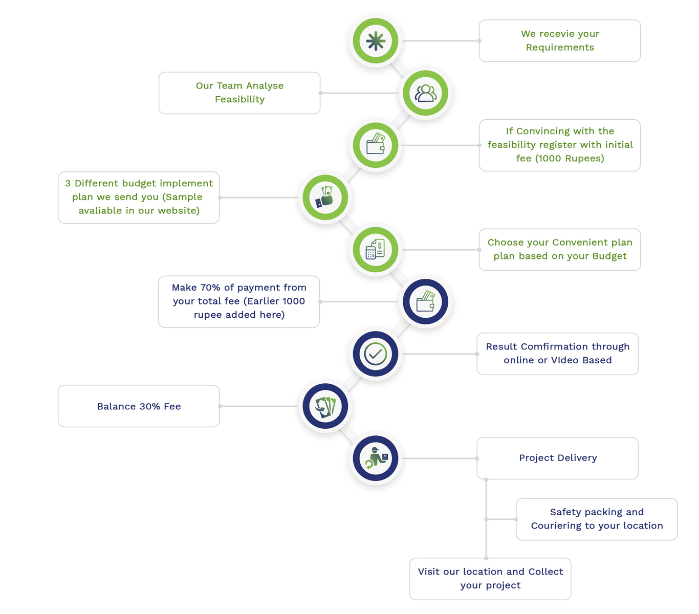
Simulation Projects Workflow
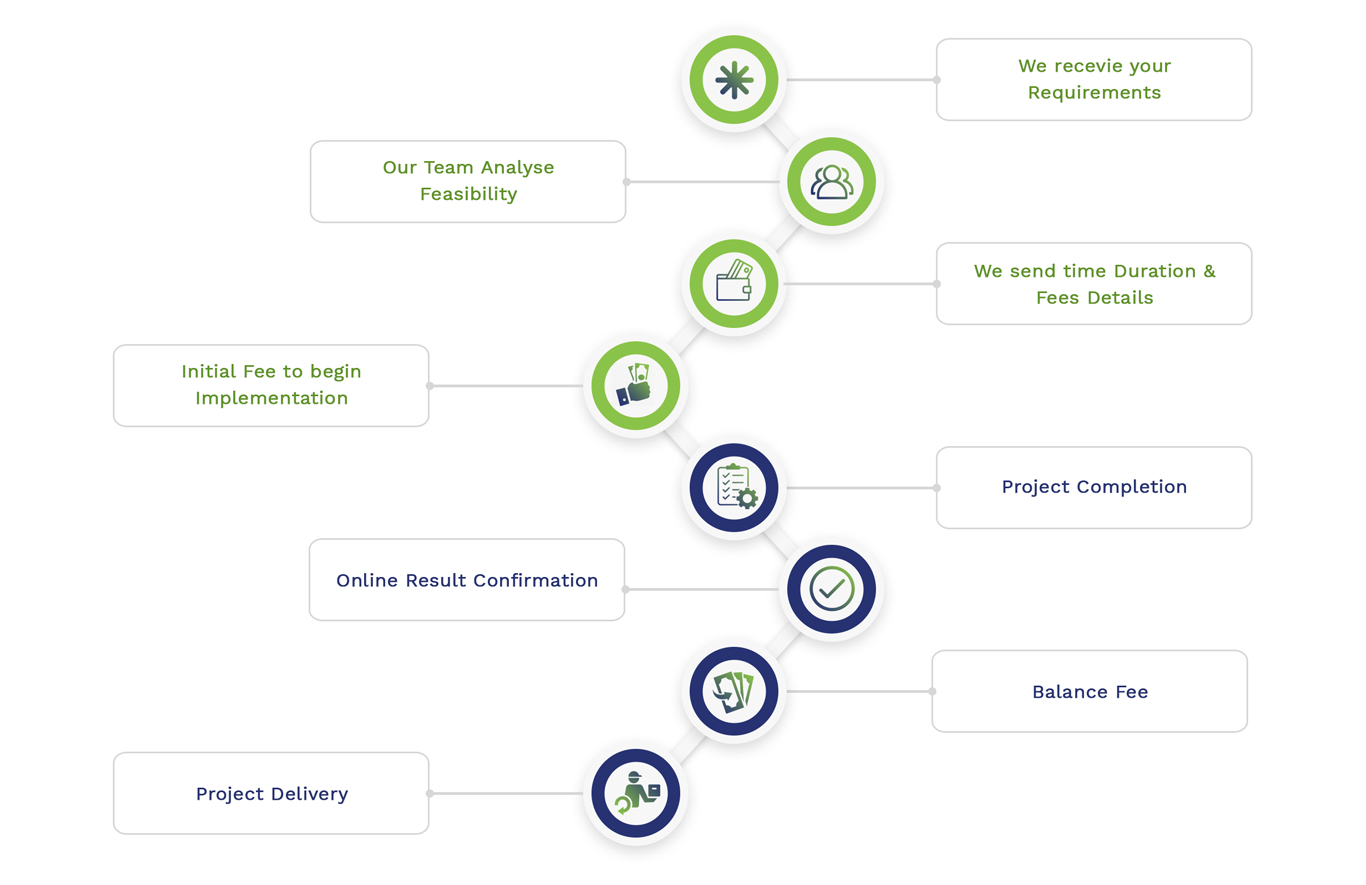
Embedded Projects Workflow