 Matlab
 Simulink
 NS3
NS3 OMNET++
 COOJA
COOJA CONTIKI OS
 NS2
NS2
Python Coding Homework Help are carried out by us in various domains such as Artificial Intelligence, Machine Learning, and Deep Learning, several projects have evolved, which are related to Python. If you are really facing difficulties then matlabprojects.org will be your trusted partner, get your work done with detailed explanation from our team. For assisting you to train and enhance your expertise, we recommend some important projects that specifically span from simple to moderate levels.
AI and Machine Learning Projects
- Linear Regression:
- By means of NumPy, a basic linear regression model has to be applied from scratch.
- In order to forecast a collection of certain data points, we employ the model.
import numpy as np
import matplotlib.pyplot as plt
# Generate some data
np.random.seed(0)
X = 2 * np.random.rand(100, 1)
y = 4 + 3 * X + np.random.randn(100, 1)
# Implement linear regression from scratch
X_b = np.c_[np.ones((100, 1)), X] # Add bias term
theta_best = np.linalg.inv(X_b.T.dot(X_b)).dot(X_b.T).dot(y)
print(“Best fit parameters:”, theta_best)
# Plot the data and the regression line
plt.scatter(X, y)
plt.plot(X, X_b.dot(theta_best), color=’red’)
plt.xlabel(“X”)
plt.ylabel(“y”)
plt.title(“Linear Regression”)
plt.show()
- Logistic Regression:
- In this project, employ NumPy to execute logistic regression from scratch.
- To a binary categorization issue, the model must be employed.
import numpy as np
from sklearn.datasets import load_breast_cancer
from sklearn.preprocessing import StandardScaler
from sklearn.model_selection import train_test_split
# Load and prepare data
data = load_breast_cancer()
X = data.data
y = data.target.reshape(-1, 1)
X_train, X_test, y_train, y_test = train_test_split(X, y, test_size=0.2, random_state=0)
scaler = StandardScaler()
X_train = scaler.fit_transform(X_train)
X_test = scaler.transform(X_test)
# Sigmoid function
def sigmoid(z):
return 1 / (1 + np.exp(-z))
# Logistic regression function
def logistic_regression(X, y, lr=0.01, iterations=1000):
m, n = X.shape
theta = np.zeros((n, 1))
for i in range(iterations):
z = X.dot(theta)
h = sigmoid(z)
gradient = X.T.dot(h – y) / m
theta -= lr * gradient
return theta
# Train model
theta = logistic_regression(X_train, y_train)
# Predict and evaluate
def predict(X, theta):
return (sigmoid(X.dot(theta)) >= 0.5).astype(int)
y_pred = predict(X_test, theta)
accuracy = np.mean(y_pred == y_test)
print(“Test accuracy:”, accuracy)
- K-Nearest Neighbors (KNN):
- From scratch, the KNN algorithm has to be applied.
- With a particular dataset, carry out a categorization problem by implementing this algorithm.
import numpy as np
from sklearn.datasets import load_iris
from sklearn.model_selection import train_test_split
from collections import Counter
# Load and prepare data
iris = load_iris()
X = iris.data
y = iris.target
X_train, X_test, y_train, y_test = train_test_split(X, y, test_size=0.2, random_state=0)
# KNN algorithm
def knn(X_train, y_train, X_test, k=3):
distances = np.sqrt(((X_train – X_test[:, np.newaxis])**2).sum(axis=2))
knn_indices = np.argsort(distances, axis=1)[:, :k]
knn_labels = y_train[knn_indices]
most_common = [Counter(labels).most_common(1)[0][0] for labels in knn_labels]
return np.array(most_common)
# Predict and evaluate
y_pred = knn(X_train, y_train, X_test, k=3)
accuracy = np.mean(y_pred == y_test)
print(“Test accuracy:”, accuracy)
Deep Learning Projects
- Neural Network from Scratch:
- Through NumPy, a basic feedforward neural network should be applied from scratch.
- Consider the XOR problem to train it.
import numpy as np
# XOR dataset
X = np.array([[0, 0], [0, 1], [1, 0], [1, 1]])
y = np.array([[0], [1], [1], [0]])
# Sigmoid activation function
def sigmoid(x):
return 1 / (1 + np.exp(-x))
# Derivative of the sigmoid function
def sigmoid_derivative(x):
return x * (1 – x)
# Initialize weights and biases
np.random.seed(0)
input_size = 2
hidden_size = 2
output_size = 1
weights_input_hidden = np.random.rand(input_size, hidden_size)
weights_hidden_output = np.random.rand(hidden_size, output_size)
bias_hidden = np.random.rand(1, hidden_size)
bias_output = np.random.rand(1, output_size)
# Training parameters
learning_rate = 0.1
epochs = 10000
# Training loop
for epoch in range(epochs):
# Forward pass
hidden_layer_input = np.dot(X, weights_input_hidden) + bias_hidden
hidden_layer_output = sigmoid(hidden_layer_input)
output_layer_input = np.dot(hidden_layer_output, weights_hidden_output) + bias_output
output_layer_output = sigmoid(output_layer_input)
# Compute the error
error = y – output_layer_output
# Backpropagation
d_output = error * sigmoid_derivative(output_layer_output)
error_hidden_layer = d_output.dot(weights_hidden_output.T)
d_hidden = error_hidden_layer * sigmoid_derivative(hidden_layer_output)
# Update weights and biases
weights_hidden_output += hidden_layer_output.T.dot(d_output) * learning_rate
bias_output += np.sum(d_output, axis=0, keepdims=True) * learning_rate
weights_input_hidden += X.T.dot(d_hidden) * learning_rate
bias_hidden += np.sum(d_hidden, axis=0, keepdims=True) * learning_rate
# Test the network
hidden_layer_input = np.dot(X, weights_input_hidden) + bias_hidden
hidden_layer_output = sigmoid(hidden_layer_input)
output_layer_input = np.dot(hidden_layer_output, weights_hidden_output) + bias_output
output_layer_output = sigmoid(output_layer_input)
print(“Predicted output:\n”, output_layer_output)
- Convolutional Neural Network (CNN) with Keras:
- By means of Keras, we develop a basic CNN. Using the MNIST dataset, the CNN must be trained.
import tensorflow as tf
from tensorflow.keras import layers, models
import matplotlib.pyplot as plt
# Load and prepare the MNIST dataset
(X_train, y_train), (X_test, y_test) = tf.keras.datasets.mnist.load_data()
X_train = X_train.reshape((X_train.shape[0], 28, 28, 1)).astype(‘float32’) / 255
X_test = X_test.reshape((X_test.shape[0], 28, 28, 1)).astype(‘float32′) / 255
# Build the CNN model
model = models.Sequential([
layers.Conv2D(32, (3, 3), activation=’relu’, input_shape=(28, 28, 1)),
layers.MaxPooling2D((2, 2)),
layers.Conv2D(64, (3, 3), activation=’relu’),
layers.MaxPooling2D((2, 2)),
layers.Conv2D(64, (3, 3), activation=’relu’),
layers.Flatten(),
layers.Dense(64, activation=’relu’),
layers.Dense(10, activation=’softmax’)
])
# Compile the model
model.compile(optimizer=’adam’,
loss=’sparse_categorical_crossentropy’,
metrics=[‘accuracy’])
# Train the model
history = model.fit(X_train, y_train, epochs=5, validation_data=(X_test, y_test))
# Evaluate the model
test_loss, test_acc = model.evaluate(X_test, y_test)
print(“Test accuracy:”, test_acc)
# Plot training history
plt.plot(history.history[‘accuracy’], label=’accuracy’)
plt.plot(history.history[‘val_accuracy’], label=’val_accuracy’)
plt.xlabel(‘Epoch’)
plt.ylabel(‘Accuracy’)
plt.legend(loc=’lower right’)
plt.show()
- Recurrent Neural Network (RNN) for Sequence Prediction:
- As a means to forecast the subsequent value in a basic series, an RNN has to be created and trained with Keras.
import numpy as np
import tensorflow as tf
from tensorflow.keras import layers, models
# Generate a simple sequence dataset
def create_sequence(n_samples=1000, n_timesteps=10):
X = np.array([i for i in range(n_samples)])
y = np.array([i + 1 for i in range(n_samples)])
X = X.reshape((n_samples, 1))
y = y.reshape((n_samples, 1))
X_seq = []
y_seq = []
for i in range(len(X) – n_timesteps):
X_seq.append(X[i:i + n_timesteps])
y_seq.append(y[i + n_timesteps])
return np.array(X_seq), np.array(y_seq)
n_timesteps = 10
X, y = create_sequence(n_timesteps=n_timesteps)
X_train, X_test = X[:800], X[800:]
y_train, y_test = y[:800], y[800:]
# Build the RNN model
model = models.Sequential([
layers.SimpleRNN(50, activation=’relu’, input_shape=(n_timesteps, 1)),
layers.Dense(1)
])
# Compile the model
model.compile(optimizer=’adam’, loss=’mse’)
# Train the model
history = model.fit(X_train, y_train, epochs=20, validation_data=(X_test, y_test))
# Predict the next value
y_pred = model.predict(X_test)
# Plot the results
import matplotlib.pyplot as plt
plt.plot(y_test, label=’True’)
plt.plot(y_pred, label=’Predicted’)
plt.xlabel(‘Time step’)
plt.ylabel(‘Value’)
plt.legend()
plt.show()
Python coding homework services
Appropriate for different fields such as Computer Science and Engineering (CSE), Electronics and Communication Engineering (ECE), Information Technology (IT), Mechanical Engineering (MECH), and Electrical and Electronics Engineering (EEE), we list out a few Python coding homework projects. For supporting students to implement Python programming to their particular domain, these projects are specifically modeled.
Computer Science and Engineering (CSE) / Information Technology (IT)
- Data Structures – Linked List Implementation:
- Including simple processes like traversal, insertion, and deletion, a singly linked list must be applied.
class Node:
def __init__(self, data):
self.data = data
self.next = None
class LinkedList:
def __init__(self):
self.head = None
def insert(self, data):
new_node = Node(data)
new_node.next = self.head
self.head = new_node
def delete(self, key):
temp = self.head
if temp is not None:
if temp.data == key:
self.head = temp.next
temp = None
return
while temp is not None:
if temp.data == key:
break
prev = temp
temp = temp.next
if temp == None:
return
prev.next = temp.next
temp = None
def print_list(self):
temp = self.head
while temp:
print(temp.data, end=’ ‘)
temp = temp.next
# Example usage
ll = LinkedList()
ll.insert(3)
ll.insert(2)
ll.insert(1)
ll.print_list() # Output: 1 2 3
ll.delete(2)
ll.print_list() # Output: 1 3
- Database Management – SQLite Integration:
- A Python script has to be developed, which carries out CRUD processes through communicating with an SQLite database.
import sqlite3
# Connect to SQLite database
conn = sqlite3.connect(‘example.db’)
cursor = conn.cursor()
# Create table
cursor.execute(”’CREATE TABLE IF NOT EXISTS students
(id INTEGER PRIMARY KEY, name TEXT, age INTEGER)”’)
# Insert data
cursor.execute(“INSERT INTO students (name, age) VALUES (‘Alice’, 21)”)
cursor.execute(“INSERT INTO students (name, age) VALUES (‘Bob’, 22)”)
# Read data
cursor.execute(“SELECT * FROM students”)
print(cursor.fetchall())
# Update data
cursor.execute(“UPDATE students SET age = 23 WHERE name = ‘Bob'”)
# Delete data
cursor.execute(“DELETE FROM students WHERE name = ‘Alice'”)
conn.commit()
conn.close()
Electronics and Communication Engineering (ECE)
- Signal Processing – Fourier Transform:
- In this project, we focus on applying the Discrete Fourier Transform (DFT). Then, the frequency elements of a signal have to be visualized.
import numpy as np
import matplotlib.pyplot as plt
# Generate a sample signal
t = np.linspace(0, 1, 500)
signal = np.sin(2 * np.pi * 5 * t) + np.sin(2 * np.pi * 20 * t)
# Compute DFT
def DFT(signal):
N = len(signal)
dft = np.zeros(N, dtype=complex)
for k in range(N):
for n in range(N):
dft[k] += signal[n] * np.exp(-2j * np.pi * k * n / N)
return dft
dft_signal = DFT(signal)
# Plot the signal and its frequency components
plt.subplot(2, 1, 1)
plt.plot(t, signal)
plt.title(‘Original Signal’)
plt.subplot(2, 1, 2)
plt.stem(np.abs(dft_signal))
plt.title(‘DFT of Signal’)
plt.show()
Electrical and Electronics Engineering (EEE)
- Circuit Analysis – Ohm’s Law Simulation:
- To simulate Ohm’s Law, a Python program should be drafted. By offering any two elements such as resistance, current, or voltage, estimate the other.
def ohms_law(voltage=None, current=None, resistance=None):
if voltage is None:
return current * resistance
elif current is None:
return voltage / resistance
elif resistance is None:
return voltage / current
# Example usage
voltage = ohms_law(current=2, resistance=5)
print(f”Voltage: {voltage} V”) # Output: Voltage: 10 V
current = ohms_law(voltage=10, resistance=5)
print(f”Current: {current} A”) # Output: Current: 2 A
resistance = ohms_law(voltage=10, current=2)
print(f”Resistance: {resistance} Ohms”) # Output: Resistance: 5 Ohms
Mechanical Engineering (MECH)
- Thermodynamics – Ideal Gas Law Simulation:
- A Python program has to be developed, which provides any two properties like volume, pressure, or temperature of a gas to estimate the other with Ideal Gas Law.
def ideal_gas_law(P=None, V=None, T=None, n=1, R=8.314):
if P is None:
return (n * R * T) / V
elif V is None:
return (n * R * T) / P
elif T is None:
return (P * V) / (n * R)
# Example usage
pressure = ideal_gas_law(V=0.1, T=300)
print(f”Pressure: {pressure} Pa”) # Output: Pressure: 2494.2 Pa
volume = ideal_gas_law(P=101325, T=300)
print(f”Volume: {volume} m^3″) # Output: Volume: 0.0246 m^3
temperature = ideal_gas_law(P=101325, V=0.0246)
print(f”Temperature: {temperature} K”) # Output: Temperature: 300.0 K
- Finite Element Analysis (FEA) – 1D Truss Analysis:
- In a truss structure, we assess the pressures and shifts by carrying out a basic 1D truss analysis.
import numpy as np
# Stiffness matrix for a 2-node 1D truss element
def stiffness_matrix(E, A, L):
return (E * A / L) * np.array([[1, -1], [-1, 1]])
# Global stiffness matrix assembly for a truss structure
def global_stiffness_matrix(elements, nodes, E, A):
n = len(nodes)
K = np.zeros((n, n))
for element in elements:
node1, node2, L = element
k = stiffness_matrix(E, A, L)
K[node1:node2+1, node1:node2+1] += k
return K
# Example truss structure
nodes = [0, 1, 2]
elements = [(0, 1, 1.0), (1, 2, 1.0)]
E = 210e9 # Young’s modulus in Pascals
A = 0.01 # Cross-sectional area in square meters
K = global_stiffness_matrix(elements, nodes, E, A)
print(“Global Stiffness Matrix:\n”, K)
For the purposes of training and knowledge enhancement, numerous intriguing projects are suggested by us. Related to various domains like CSE, ECE, IT, MECH, and EEE, we proposed several Python coding homework projects, along with concise explanations.
Subscribe Our Youtube Channel
You can Watch all Subjects Matlab & Simulink latest Innovative Project Results

Our services
We want to support Uncompromise Matlab service for all your Requirements Our Reseachers and Technical team keep update the technology for all subjects ,We assure We Meet out Your Needs.
Our Services
- Matlab Research Paper Help
- Matlab assignment help
- Matlab Project Help
- Matlab Homework Help
- Simulink assignment help
- Simulink Project Help
- Simulink Homework Help
- Matlab Research Paper Help
- NS3 Research Paper Help
- Omnet++ Research Paper Help
Our Benefits
- Customised Matlab Assignments
- Global Assignment Knowledge
- Best Assignment Writers
- Certified Matlab Trainers
- Experienced Matlab Developers
- Over 400k+ Satisfied Students
- Ontime support
- Best Price Guarantee
- Plagiarism Free Work
- Correct Citations
Expert Matlab services just 1-click

Delivery Materials
Unlimited support we offer you
For better understanding purpose we provide following Materials for all Kind of Research & Assignment & Homework service.
 Programs
 Designs
 Simulations
 Results
 Graphs
 Result snapshot
 Video Tutorial
 Instructions Profile
  Sofware Install Guide
 Execution Guidance
  Explanations
 Implement Plan
Matlab Projects
Matlab projects innovators has laid our steps in all dimension related to math works.Our concern support matlab projects for more than 10 years.Many Research scholars are benefited by our matlab projects service.We are trusted institution who supplies matlab projects for many universities and colleges.
Reasons to choose Matlab Projects .org???
Our Service are widely utilized by Research centers.More than 5000+ Projects & Thesis has been provided by us to Students & Research Scholars. All current mathworks software versions are being updated by us.
Our concern has provided the required solution for all the above mention technical problems required by clients with best Customer Support.
- Novel Idea
- Ontime Delivery
- Best Prices
- Unique Work
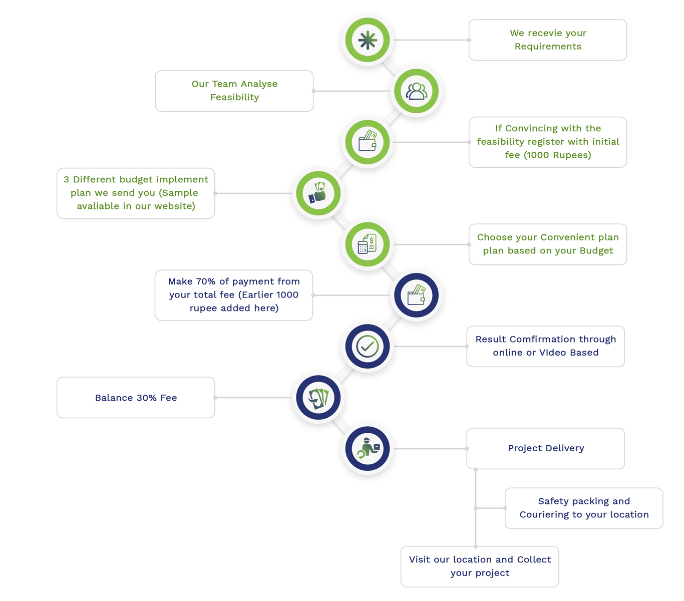
Simulation Projects Workflow

Embedded Projects Workflow