 Matlab
 Simulink
 NS3
NS3 OMNET++
 COOJA
COOJA CONTIKI OS
 NS2
NS2
MATLAB Programming Help across all areas are done by us, if you are keen looking for novel ideas and best writers’ assistance then we will be your first priority. Across various research fields, MATLAB programming is utilized in an extensive way for several purposes. Regarding in what way MATLAB programming can assist in different research fields, we offer an explicit instruction, including particular instances:
- Machine Learning and Data Science
Instance: Linear Regression
% Load data
data = load(‘data.mat’);
X = data.X;
y = data.y;
% Add intercept term
X = [ones(size(X, 1), 1) X];
% Calculate parameters using the normal equation
theta = (X’ * X) \ (X’ * y);
% Predict values
predictions = X * theta;
% Plot results
figure;
scatter(X(:, 2), y);
hold on;
plot(X(:, 2), predictions, ‘-r’);
xlabel(‘Feature’);
ylabel(‘Target’);
title(‘Linear Regression’);
- Signal Processing
Instance: Fourier Transform
% Generate a signal
Fs = 1000; % Sampling frequency
T = 1/Fs; % Sampling period
L = 1000; % Length of signal
t = (0:L-1)*T; % Time vector
S = 0.7*sin(2*pi*50*t) + sin(2*pi*120*t); % Signal
% Compute the Fourier Transform
Y = fft(S);
% Compute the two-sided spectrum P2
P2 = abs(Y/L);
P1 = P2(1:L/2+1);
P1(2:end-1) = 2*P1(2:end-1);
% Define the frequency domain f
f = Fs*(0:(L/2))/L;
% Plot the single-sided amplitude spectrum
figure;
plot(f,P1)
title(‘Single-Sided Amplitude Spectrum of S(t)’)
xlabel(‘f (Hz)’)
ylabel(‘|P1(f)|’)
- Control Systems
Instance: PID Controller
% Define the transfer function
s = tf(‘s’);
G = 1 / (s^2 + 10*s + 20);
% Define the PID controller
Kp = 300;
Ki = 70;
Kd = 50;
C = pid(Kp, Ki, Kd);
% Open-loop transfer function
T = feedback(C*G, 1);
% Plot step response
figure;
step(T);
title(‘Step Response with PID Controller’);
- Image Processing
Instance: Edge Detection
% Read the image
I = imread(‘image.jpg’);
% Convert to grayscale
I_gray = rgb2gray(I);
% Apply edge detection
edges = edge(I_gray, ‘Canny’);
% Display the original image and edges
figure;
subplot(1, 2, 1);
imshow(I);
title(‘Original Image’);
subplot(1, 2, 2);
imshow(edges);
title(‘Edge Detection’);
- Optimization
Instance: Utilizing fmincon for Constrained Optimization
% Define the objective function
objective = @(x) (x(1) – 2)^2 + (x(2) – 3)^2;
% Initial guess
x0 = [0, 0];
% Constraints
A = []; b = [];
Aeq = []; beq = [];
lb = [0, 0];
ub = [5, 5];
nonlcon = [];
% Solve the problem
[x_opt, fval] = fmincon(objective, x0, A, b, Aeq, beq, lb, ub, nonlcon);
% Display results
fprintf(‘Optimal solution: x1 = %f, x2 = %f\n’, x_opt(1), x_opt(2));
fprintf(‘Optimal objective value: %f\n’, fval);
- Financial Modeling
Instance: Black-Scholes Option Pricing
% Parameters
S = 100; % Stock price
K = 100; % Strike price
r = 0.05; % Risk-free rate
T = 1; % Time to maturity
sigma = 0.2; % Volatility
% Calculate d1 and d2
d1 = (log(S/K) + (r + sigma^2 / 2) * T) / (sigma * sqrt(T));
d2 = d1 – sigma * sqrt(T);
% Calculate the call and put option prices
call_price = S * normcdf(d1) – K * exp(-r * T) * normcdf(d2);
put_price = K * exp(-r * T) * normcdf(-d2) – S * normcdf(-d1);
% Display results
fprintf(‘Call Option Price: %f\n’, call_price);
fprintf(‘Put Option Price: %f\n’, put_price);
- Robotics
Instance: Inverse Kinematics for a 2-DOF Manipulator
% Parameters
L1 = 1; % Length of first arm
L2 = 1; % Length of second arm
x = 1; % Target x position
y = 1; % Target y position
% Inverse Kinematics calculations
cos_theta2 = (x^2 + y^2 – L1^2 – L2^2) / (2 * L1 * L2);
sin_theta2 = sqrt(1 – cos_theta2^2);
theta2 = atan2(sin_theta2, cos_theta2);
k1 = L1 + L2 * cos(theta2);
k2 = L2 * sin(theta2);
theta1 = atan2(y, x) – atan2(k2, k1);
% Display results
fprintf(‘Theta1: %f radians\n’, theta1);
fprintf(‘Theta2: %f radians\n’, theta2);
- Renewable Energy
Instance: Designing a Solar PV System
% Parameters
Isc = 5; % Short-circuit current
Voc = 20; % Open-circuit voltage
n = 1.2; % Diode ideality factor
Rs = 0.1; % Series resistance
Rp = 100; % Parallel resistance
T = 25 + 273.15; % Temperature in Kelvin
k = 1.38e-23; % Boltzmann constant
q = 1.6e-19; % Electron charge
% Calculate I-V curve
V = linspace(0, Voc, 100);
I = zeros(size(V));
for i = 1:length(V)
I(i) = Isc – Isc * (exp((q * (V(i) + I(i) * Rs)) / (n * k * T)) – 1) – (V(i) + I(i) * Rs) / Rp;
end
% Plot the I-V curve
figure;
plot(V, I, ‘LineWidth’, 2);
xlabel(‘Voltage (V)’);
ylabel(‘Current (I)’);
title(‘I-V Curve of Solar PV System’);
grid on;
Matlab programming help for Comparative analysis
Carrying out a comparative analysis with MATLAB is an intriguing as well as challenging process. Based on performing a comparative analysis with MATLAB, we provide an in-depth procedural instruction. For comparing machine learning models and optimization algorithms, some important samples are offered by us:
Sample 1: Comparative Analysis of Optimization Algorithms
On a basic quadratic function, the performance of Particle Swarm Optimization (PSO) and Gradient Descent has to be compared.
Step 1: Specify the Optimization Issue
function y = objective_function(x)
y = (x – 3)^2;
end
Step 2: Apply Optimization Algorithms
Gradient Descent:
function [x, fval, iter] = gradient_descent(alpha, tol, max_iter)
x = 0;
iter = 0;
grad = @(x) 2 * (x – 3);
while iter < max_iter
iter = iter + 1;
grad_val = grad(x);
x_new = x – alpha * grad_val;
if abs(x_new – x) < tol
break;
end
x = x_new;
end
fval = objective_function(x);
end
Particle Swarm Optimization (PSO):
function [global_best, fval] = particle_swarm_optimization(num_particles, max_iter, w, c1, c2)
particles = rand(num_particles, 1) * 10 – 5;
velocities = zeros(num_particles, 1);
personal_best = particles;
personal_best_fval = arrayfun(@objective_function, particles);
[global_best_fval, idx] = min(personal_best_fval);
global_best = personal_best(idx);
for iter = 1:max_iter
for i = 1:num_particles
r1 = rand();
r2 = rand();
velocities(i) = w * velocities(i) + c1 * r1 * (personal_best(i) – particles(i)) + c2 * r2 * (global_best – particles(i));
particles(i) = particles(i) + velocities(i);
fval = objective_function(particles(i));
if fval < personal_best_fval(i)
personal_best(i) = particles(i);
personal_best_fval(i) = fval;
end
end
[current_global_best_fval, idx] = min(personal_best_fval);
if current_global_best_fval < global_best_fval
global_best_fval = current_global_best_fval;
global_best = personal_best(idx);
end
end
fval = global_best_fval;
end
Step 3: Set Parameters
% Parameters for Gradient Descent
alpha = 0.1;
tol = 1e-6;
max_iter = 1000;
% Parameters for PSO
num_particles = 30;
max_iter_pso = 100;
w = 0.5;
c1 = 1.5;
c2 = 1.5;
Step 4: Execute the Algorithms
% Gradient Descent
[x_gd, fval_gd, iter_gd] = gradient_descent(alpha, tol, max_iter);
% Particle Swarm Optimization
[x_pso, fval_pso] = particle_swarm_optimization(num_particles, max_iter_pso, w, c1, c2);
% Display results
fprintf(‘Gradient Descent: Optimal x = %f, fval = %f, iterations = %d\n’, x_gd, fval_gd, iter_gd);
fprintf(‘Particle Swarm Optimization: Optimal x = %f, fval = %f\n’, x_pso, fval_pso);
Step 5: Examine Outcomes
% Plot the function
f = @(x) (x – 3)^2;
x_vals = linspace(-2, 8, 100);
y_vals = f(x_vals);
figure;
plot(x_vals, y_vals, ‘LineWidth’, 2);
hold on;
plot(x_gd, fval_gd, ‘ro’, ‘MarkerSize’, 10, ‘MarkerFaceColor’, ‘r’);
plot(x_pso, fval_pso, ‘bo’, ‘MarkerSize’, 10, ‘MarkerFaceColor’, ‘b’);
xlabel(‘x’);
ylabel(‘f(x)’);
title(‘Optimization Results’);
legend(‘Objective Function’, ‘Gradient Descent’, ‘PSO’);
grid on;
Sample 2: Comparative Analysis of Machine Learning Models
For a categorization issue, we compare the performance of Support Vector Machine (SVM) and Logistic Regression.
Step 1: Load Data
load fisheriris;
X = meas(:, 1:2); % Use only first two features for simplicity
y = species;
Step 2: Divide Data into Training and Test Sets
cv = cvpartition(y, ‘HoldOut’, 0.3);
X_train = X(training(cv), :);
y_train = y(training(cv), :);
X_test = X(test(cv), :);
y_test = y(test(cv), :);
Step 3: Train and Assess Models
Logistic Regression:
logistic_model = fitclinear(X_train, y_train, ‘Learner’, ‘logistic’);
y_pred_logistic = predict(logistic_model, X_test);
accuracy_logistic = sum(strcmp(y_pred_logistic, y_test)) / length(y_test);
Support Vector Machine (SVM):
svm_model = fitcsvm(X_train, y_train);
y_pred_svm = predict(svm_model, X_test);
accuracy_svm = sum(strcmp(y_pred_svm, y_test)) / length(y_test);
Step 4: Depict Outcomes
fprintf(‘Logistic Regression Accuracy: %.2f%%\n’, accuracy_logistic * 100);
fprintf(‘SVM Accuracy: %.2f%%\n’, accuracy_svm * 100);
Step 5: Visualize Outcomes
figure;
% Logistic Regression
subplot(1, 2, 1);
gscatter(X_test(:,1), X_test(:,2), y_pred_logistic, ‘rgb’, ‘osd’);
title(‘Logistic Regression’);
xlabel(‘Feature 1’);
ylabel(‘Feature 2’);
% SVM
subplot(1, 2, 2);
gscatter(X_test(:,1), X_test(:,2), y_pred_svm, ‘rgb’, ‘osd’);
title(‘SVM’);
xlabel(‘Feature 1’);
ylabel(‘Feature 2’);
By considering how MATLAB programming can assist in different research fields, we suggested a thorough instruction, along with some particular samples. If you are confused on any level of MATLAB project, be free to get our Programming Help. To carry out a comparative analysis with MATLAB, procedural guidelines are provided by us, encompassing a few major instances. Be in touch with us for getting novel results.
Subscribe Our Youtube Channel
You can Watch all Subjects Matlab & Simulink latest Innovative Project Results

Our services
We want to support Uncompromise Matlab service for all your Requirements Our Reseachers and Technical team keep update the technology for all subjects ,We assure We Meet out Your Needs.
Our Services
- Matlab Research Paper Help
- Matlab assignment help
- Matlab Project Help
- Matlab Homework Help
- Simulink assignment help
- Simulink Project Help
- Simulink Homework Help
- Matlab Research Paper Help
- NS3 Research Paper Help
- Omnet++ Research Paper Help
Our Benefits
- Customised Matlab Assignments
- Global Assignment Knowledge
- Best Assignment Writers
- Certified Matlab Trainers
- Experienced Matlab Developers
- Over 400k+ Satisfied Students
- Ontime support
- Best Price Guarantee
- Plagiarism Free Work
- Correct Citations
Expert Matlab services just 1-click

Delivery Materials
Unlimited support we offer you
For better understanding purpose we provide following Materials for all Kind of Research & Assignment & Homework service.
 Programs
 Designs
 Simulations
 Results
 Graphs
 Result snapshot
 Video Tutorial
 Instructions Profile
  Sofware Install Guide
 Execution Guidance
  Explanations
 Implement Plan
Matlab Projects
Matlab projects innovators has laid our steps in all dimension related to math works.Our concern support matlab projects for more than 10 years.Many Research scholars are benefited by our matlab projects service.We are trusted institution who supplies matlab projects for many universities and colleges.
Reasons to choose Matlab Projects .org???
Our Service are widely utilized by Research centers.More than 5000+ Projects & Thesis has been provided by us to Students & Research Scholars. All current mathworks software versions are being updated by us.
Our concern has provided the required solution for all the above mention technical problems required by clients with best Customer Support.
- Novel Idea
- Ontime Delivery
- Best Prices
- Unique Work
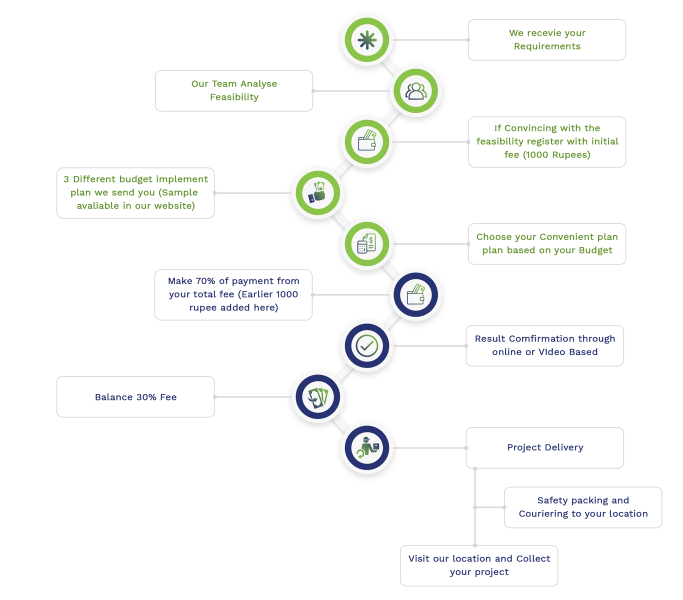
Simulation Projects Workflow
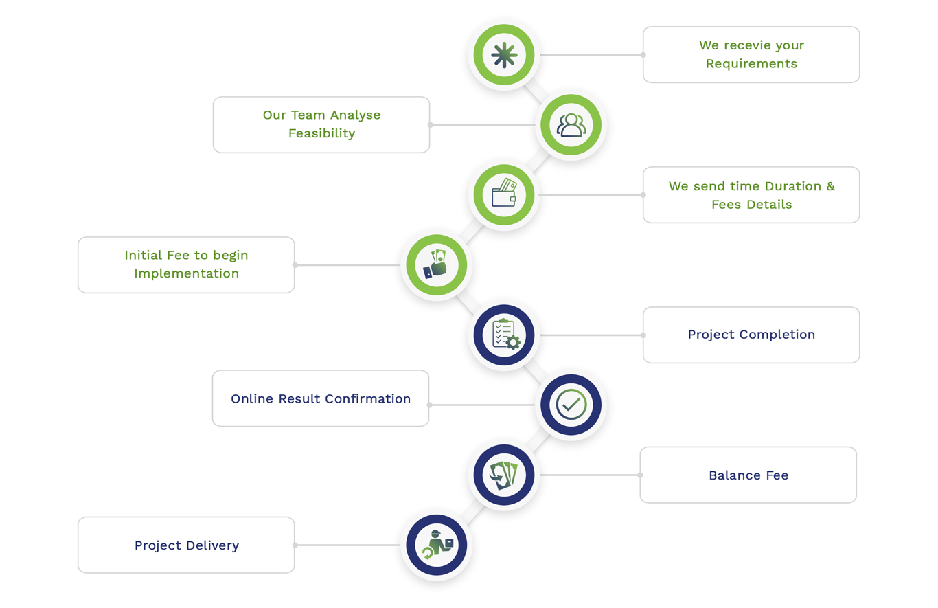
Embedded Projects Workflow