 Matlab
 Simulink
 NS3
NS3 OMNET++
 COOJA
COOJA CONTIKI OS
 NS2
NS2
Gradient Descent in MATLAB includes diverse tools that can be useful for addressing complicated programs. We have a well-trained team of researchers and developers who work on all leading tools and algorithms .Get tailored simulation services from us. To execute gradient descent for optimization issues, we provide an extensive guide.
To execute gradient descent in MATLAB, manual explanation is offered here:
Step-by-Step Procedure
- Specify the Objective Function
The function which we aim to decrease needs to be specified as an objective function. It might be a cost function or arithmetical function for a machine learning framework.
- Evaluate the Gradient
Path of the steepest descent should be defined by the gradient of the objective function.
- Execute Gradient Descent
Initiate the parameters and determine the adaptive learning rate to configure gradient descent algorithm. For upgrading the parameters, repeat this procedure.
Instance: Gradient Descent for a Basic Quadratic Function
To reduce the following quadratic function: f(x) =x2+4sin(x) f(x) = x^2 + 4\sin(x) f(x) =x2+4sin(x), consider the following measures:
Step 1: Determine the Objective Function
A MATLAB function file need to be designed (For ex: objectiveFunction.m):
function y = objectiveFunction(x)
y = x.^2 + 4*sin(x);
end
Step 2: Evaluate the Gradient
For the gradient of the objective function such as (gradientFunction.m), a MATLAB function file is required to be modeled:
function g = gradientFunction(x)
g = 2*x + 4*cos(x);
end
Step 3: Execute Gradient Descent
% Parameters for gradient descent
learningRate = 0.01;
maxIterations = 1000;
tolerance = 1e-6;
% Initialize x
x = 10; % Starting point
history = zeros(maxIterations, 1); % To store the value of the objective function
% Gradient descent loop
for i = 1:maxIterations
% Compute the gradient
grad = gradientFunction(x);
% Update x
x = x – learningRate * grad;
% Save the objective function value
history(i) = objectiveFunction(x);
% Check for convergence
if abs(grad) < tolerance
fprintf(‘Converged in %d iterations\n’, i);
break;
end
end
% Trim the history array
history = history(1:i);
% Display the result
disp([‘Optimal x: ‘, num2str(x)]);
disp([‘Optimal value: ‘, num2str(objectiveFunction(x))]);
% Plot the objective function value over iterations
figure;
plot(1:i, history, ‘LineWidth’, 2);
xlabel(‘Iteration’);
ylabel(‘Objective Function Value’);
title(‘Gradient Descent Convergence’);
grid on;
Explanation
- Initialization: Initially, we have to determine the learning rate and considerable number of executions. For convergence, specify the forbearance. To a beginning point, set x.
- Gradient Descent Loop: Evaluate the gradient of the objective function at each cycle, move in the direction which is contrary to the gradient for upgrading x and the objective function valued must be saved by us. Contrast the magnitude of the gradient with the forbearance to verify the integration.
- Outcome: The approximate value of x and consistent value of objective function ought to be exhibited. To visualize the synthesization, the objective function must be designed across replications.
Further Circumstances
- Selecting the Learning Rate: Considering each iteration, the learning rate handles the convergence rate. The integration will be slow in the case of insufficient and if it’s very extensive, the technique might deviate. As regards various learning rates, we have to conduct practical experimentation.
- Stopping Criteria: We can deploy the modifications in a determined range of iterations as stopping criteria or the value of objective function, apart from the magnitude of gradients.
- Momentum and Adaptive Techniques: The variations of gradient descent like Adam, RMSprop and momentum should be executed for enhancing the integration.
Instance with Built-in MATLAB Function
Especially for optimization, MATLAB also offers built-in functions like finance that effectively deploys techniques of gradients.
% Define the objective function
objective = @objectiveFunction;
% Define the gradient function
options = optimoptions(‘fminunc’, ‘GradObj’, ‘on’, ‘Display’, ‘iter’);
% Run the optimization
[x, fval] = fminunc(objective, 10, options);
% Display the results
disp([‘Optimal x: ‘, num2str(x)]);
disp([‘Optimal value: ‘, num2str(fval)]);
The gradient computation and optimization process is efficiently managed in an automatic manner by using the fminunc in this instance. MATLAB can approach it mathematically or we can define the gradient by using the ‘GradObj’ option.
Top 50 gradient descent algorithms list
Gradient descent is a crucial optimization technique which is typically deployed to train neural networks and machine learning models. For addressing the optimization problem, lists of 50 significant gradient descent techniques are offered by us:
Simple Gradient Descent Algorithms
- Stochastic Gradient Descent (SGD)
- Vanilla Gradient Descent
- Mini-Batch Gradient Descent
- Batch Gradient Descent
Gradient Descent with Momentum
- Nesterov Accelerated Gradient (NAG)
- Momentum Gradient Descent
Adaptive Learning Rate Methods
- Adam (Adaptive Moment Estimation)
- Nadam (Nesterov-accelerated Adam)
- Adadelta
- RMSprop (Root Mean Square Propagation)
- AMSGrad
- Adagrad (Adaptive Gradient Algorithm)
Second-Order Methods
- Limited-memory BFGS (L-BFGS)
- Broyden-Fletcher-Goldfarb-Shanno (BFGS) Algorithm
- Newton’s Method
- Hessian-Free Optimization
- Quasi-Newton Method
Variants Based on Line Search
- Armijo Rule
- Backtracking Line Search
- Wolfe Conditions
Conjugate Gradient Methods
- Hestenes-Stiefel Conjugate Gradient
- Fletcher-Reeves Conjugate Gradient
- Polak-Ribiere Conjugate Gradient
Coordinate Descent Methods
- Randomized Coordinate Descent
- Coordinate Gradient
Hybrid Methods
- Gradient Descent with Line Search
- Gradient Descent with Conjugate Gradient
- Hybrid L-BFGS
Proximal Gradient Methods
- Accelerated Proximal Gradient
- Proximal Gradient Descent
Variants for Deep Learning
- Cyclical Learning Rate (CLR)
- Stochastic Weight Averaging (SWA)
- Layer-wise Adaptive Rate Scaling (LARS)
- Gradient Clipping
- Lookahead Optimizer
Robustness and Stability Methods
- Gradient Descent with Dropout
- Gradient Descent with Regularization (L1, L2)
- Gradient Descent with Early Stopping
Distributed and Parallel Methods
- Elastic Averaging SGD (EASGD)
- Distributed Gradient Descent
- Federated Averaging (FedAvg)
Other Variants and Enhancements
- Stochastic Variance Reduced Gradient (SVRG)
- Proximal Policy Optimization (PPO)
- Normalized Gradient Descent
- Accelerated Gradient Descent
- Heavy Ball Method
- Frank-Wolfe Algorithm
- Projected Gradient Descent
- Mirror Descent
- Subgradient Descent
Brief Description of Critical Algorithms
- Batch Gradient Descent: For the overall training data set, this technique evaluates the gradients of the cost function on the basis of constraints.
- Stochastic Gradient Descent (SGD): Considering the specific training framework enhances the parameters. As a result, rapid convergence and extensive frequent upgrades are occurred.
- Mini-Batch Gradient Descent: The training datasets are classified into small branches in this technique. For each batch, it carries out an update. Advantages of both batch and stochastic methods are effectively stabilized here.
- Momentum Gradient Descent: In order to speed up the convergence, this method incorporates a fraction of the initial update vector to the existing update vector.
- Nesterov Accelerated Gradient (NAG): It includes feedforward measures to enhance momentum.
- Adagrad: Depending on the past records of gradient data, the learning rate of each parameter can be adjusted by this method.
- RMSprop: By means of utilizing a simple moving average of squared gradients, the reducing learning rates in Adagrad can be mentioned through this technique.
- Adam: As regards specific parameters, this technique evaluates the adaptive learning rates through integrating the benefits of Adagrad as well as RMSprop.
- Newton’s Method: For upgrading the parameters, it effectively uses the Hessian matrix and regarding well-mannered functions, this method offers rapid integration.
- BFGS and L-BFGS: To enhance the parameters in an effective manner, it deploys Quasi-Newton techniques which estimate the Hessian matrix.
- Fletcher-Reeves and Polak-Ribiere Conjugate Gradient: Specifically for extensive and effective optimization, we should make use of conjugate directions instead of gradients
- Coordinate Gradient Descent: For solving the optimization issue, this method upgrades one coordinate (parameter) consequently.
- Proximal Gradient Descent: To manage complicated functions, this method integrates gradient descent with a proximal operator.
- Layer-wise Adaptive Rate Scaling (LARS): Regarding each layer in deep networks, it adjusts the adaptive learning rates.
- Lookahead Optimizer: It effectively preserves two sets of parameters for optimizing the flexibility and functionality.
- Gradient Descent with Early Stopping: While the effectiveness on a validation set begins to reduce, it avoids overfitting through terminating the process of training.
- Federated Averaging (FedAvg): In federated learning, this technique accumulates model upgrades from diverse devices.
MATLAB is a highly applicable programming language among users and developers, as it is a user-friendly interface. In the motive of assisting you in executing gradient descent in MATLAB, we provide simple steps with some trending and impactful techniques.
Our team assists you in tackling complex programs related to Gradient Descent in MATLAB, utilizing a variety of tools to deliver optimal results. Share with us all your reasech needs to get tailored services from our experts.
Subscribe Our Youtube Channel
You can Watch all Subjects Matlab & Simulink latest Innovative Project Results

Our services
We want to support Uncompromise Matlab service for all your Requirements Our Reseachers and Technical team keep update the technology for all subjects ,We assure We Meet out Your Needs.
Our Services
- Matlab Research Paper Help
- Matlab assignment help
- Matlab Project Help
- Matlab Homework Help
- Simulink assignment help
- Simulink Project Help
- Simulink Homework Help
- Matlab Research Paper Help
- NS3 Research Paper Help
- Omnet++ Research Paper Help
Our Benefits
- Customised Matlab Assignments
- Global Assignment Knowledge
- Best Assignment Writers
- Certified Matlab Trainers
- Experienced Matlab Developers
- Over 400k+ Satisfied Students
- Ontime support
- Best Price Guarantee
- Plagiarism Free Work
- Correct Citations
Expert Matlab services just 1-click

Delivery Materials
Unlimited support we offer you
For better understanding purpose we provide following Materials for all Kind of Research & Assignment & Homework service.
 Programs
 Designs
 Simulations
 Results
 Graphs
 Result snapshot
 Video Tutorial
 Instructions Profile
  Sofware Install Guide
 Execution Guidance
  Explanations
 Implement Plan
Matlab Projects
Matlab projects innovators has laid our steps in all dimension related to math works.Our concern support matlab projects for more than 10 years.Many Research scholars are benefited by our matlab projects service.We are trusted institution who supplies matlab projects for many universities and colleges.
Reasons to choose Matlab Projects .org???
Our Service are widely utilized by Research centers.More than 5000+ Projects & Thesis has been provided by us to Students & Research Scholars. All current mathworks software versions are being updated by us.
Our concern has provided the required solution for all the above mention technical problems required by clients with best Customer Support.
- Novel Idea
- Ontime Delivery
- Best Prices
- Unique Work
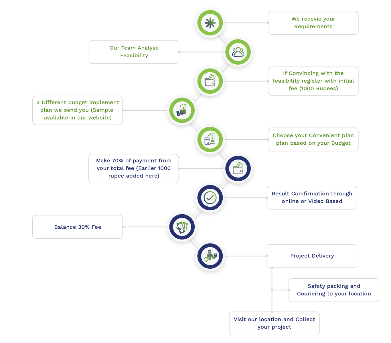
Simulation Projects Workflow
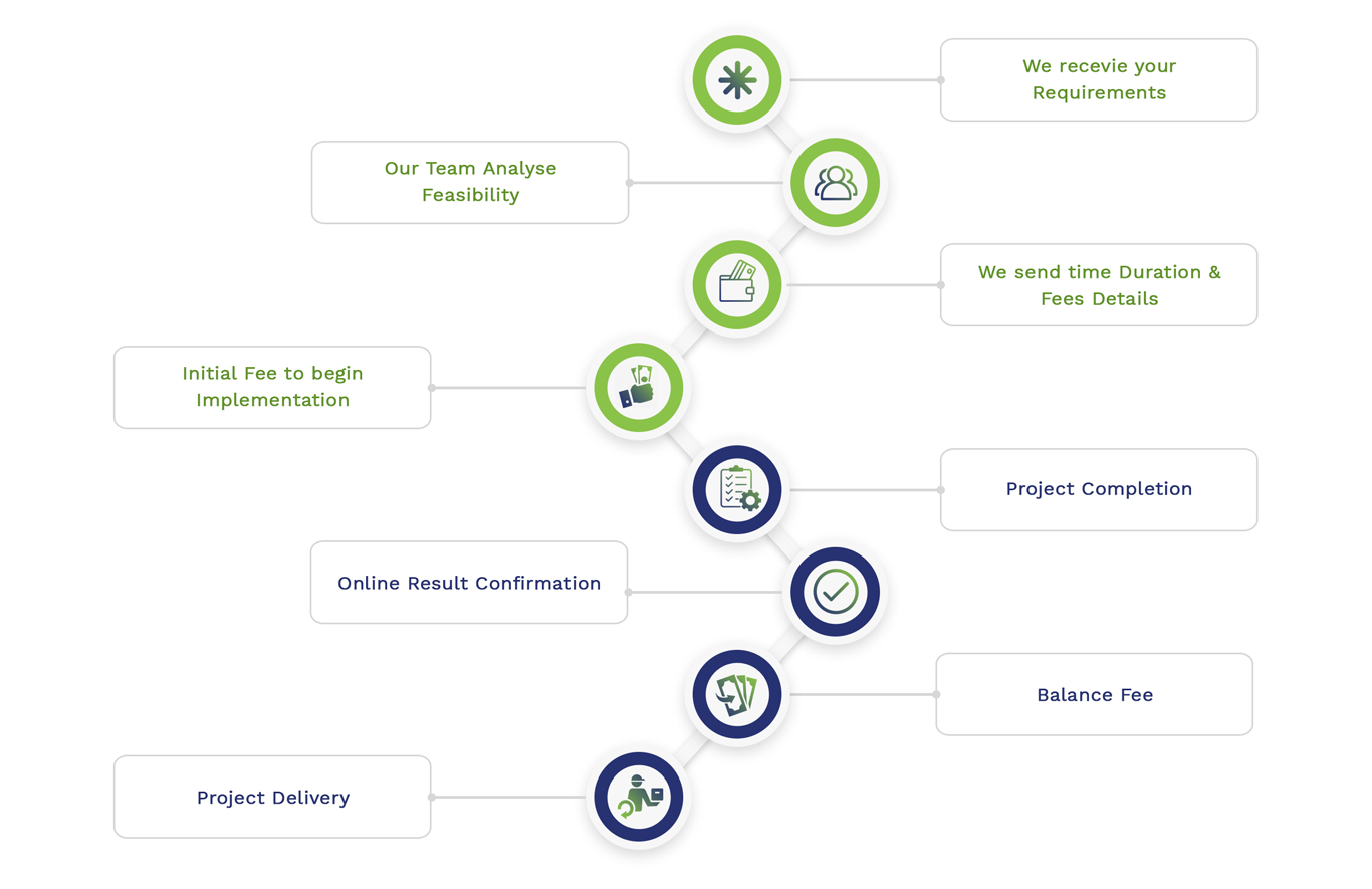
Embedded Projects Workflow