 Matlab
 Simulink
 NS3
NS3 OMNET++
 COOJA
COOJA CONTIKI OS
 NS2
NS2
MATLAB Assistance for all types of scholars across all levels are aided by us. Across several areas, some of the considerable and existing research problems are provided by us. If you share with us you project details we will give you novel services. On all areas of MATLAB we are ready to guide you with our leading researchers. To aid you in managing these issues, efficient MATLAB code snippets with simple manual procedures are addressed here.
Research Problem 1: Predictive Maintenance Using Machine Learning
Aim:
To anticipate machine breakdown, a predictive maintenance system ought to be created which efficiently deploys past records of sensor data.
Measures:
- Data Preprocessing
- Feature Extraction
- Model Training
- Model Assessment
MATLAB Code:
% Load and preprocess data
data = readtable(‘machine_data.csv’);
data = rmmissing(data); % Remove missing values
% Feature extraction
X = data{:, 1:end-1}; % Features
y = data{:, end}; % Labels (0 for no failure, 1 for failure)
% Split data into training and testing sets
cv = cvpartition(y, ‘HoldOut’, 0.3);
XTrain = X(training(cv), :);
yTrain = y(training(cv));
XTest = X(test(cv), :);
yTest = y(test(cv));
% Train a machine learning model (e.g., SVM)
model = fitcsvm(XTrain, yTrain);
% Evaluate the model
predictions = predict(model, XTest);
accuracy = sum(predictions == yTest) / numel(yTest);
disp([‘Accuracy: ‘, num2str(accuracy * 100), ‘%’]);
Research Problem 2: Adaptive Noise Cancellation in Audio Signals
Aim:
Make use of LMS (Least Mean Squares) technique to separate noise from an audio signal.
Measures:
- Import Audio Signals
- Execute LMS Algorithm
- Assess Performance
MATLAB Code:
% Load audio signals
[desiredSignal, Fs] = audioread(‘clean_audio.wav’);
[noiseSignal, ~] = audioread(‘noise.wav’);
% Create noisy signal
noisySignal = desiredSignal + noiseSignal;
% Parameters for LMS
mu = 0.01; % Step size
filterOrder = 32; % Number of filter coefficients
% Initialize variables
w = zeros(filterOrder, 1);
y = zeros(length(noisySignal), 1);
e = zeros(length(noisySignal), 1);
% LMS Algorithm
for n = filterOrder:length(noisySignal)
x = noiseSignal(n:-1:n-filterOrder+1);
y(n) = w’ * x;
e(n) = noisySignal(n) – y(n);
w = w + mu * x * e(n);
end
% Plot results
figure;
subplot(2, 1, 1);
plot(noisySignal);
title(‘Noisy Signal’);
subplot(2, 1, 2);
plot(e);
title(‘Cleaned Signal using LMS’);
Research Problem 3: Image Segmentation Using K-means Clustering
Aim:
By using K-means clustering, we must classify an image into various areas.
Measures:
- Import and Preprocess Image
- Implement K-means Clustering
- Visualize Segmented Image
MATLAB Code:
% Load image
img = imread(‘peppers.png’);
figure;
imshow(img);
title(‘Original Image’);
% Reshape image into 2D array
pixelData = double(reshape(img, [], 3));
% Apply K-means clustering
K = 3; % Number of clusters
[idx, C] = kmeans(pixelData, K);
% Map each pixel to the centroid color
segmentedImg = reshape(C(idx, :), size(img));
% Display segmented image
figure;
imshow(uint8(segmentedImg));
title(‘Segmented Image’);
Research Problem 4: Control of an Inverted Pendulum Using PID
Aim:
For stabilizing an inverted pendulum, a PID controller needs to be modeled in an efficient manner.
Measures:
- Specify System Dynamics
- Develop PID Controller
- Simulate System
MATLAB Code:
% define system parameters
m = 0.5; % Mass of pendulum
L = 0.3; % Length of pendulum
g = 9.81; % Acceleration due to gravity
b = 0.1; % Damping coefficient
% State-space representation
A = [0 1 0 0; 0 -b/m g/L 0; 0 0 0 1; 0 -b/(m*L) g/(m*L) 0];
B = [0; 1/m; 0; 1/(m*L)];
C = [1 0 0 0];
D = 0;
% PID controller design
Kp = 100;
Ki = 1;
Kd = 20;
pid_controller = pid(Kp, Ki, Kd);
% Create state-space model and closed-loop system
sys = ss(A, B, C, D);
cl_sys = feedback(pid_controller*sys, 1);
% Simulate step response
step(cl_sys);
title(‘Step Response with PID Controller’);
Research Problem 5: Predicting Stock Prices Using Time Series Analysis
Aim:
We must anticipate the upcoming stock prices through creating a time series framework.
Measures:
- Import Stock Price Data
- Preprocess Data
- Fit ARIMA Model
- Predict Upcoming Prices
MATLAB Code:
% Load stock price data
data = readtable(‘stock_prices.csv’);
prices = data.Close;
dates = data.Date;
% Convert to time series object
ts = timeseries(prices, dates);
% Plot the data
figure;
plot(ts.Time, ts.Data);
title(‘Stock Prices’);
xlabel(‘Date’);
ylabel(‘Price’);
% Fit ARIMA model
model = arima(‘Constant’, 0, ‘D’, 1, ‘Seasonality’, 12, ‘MALags’, 1, ‘SMALags’, 12);
fit = estimate(model, ts.Data);
% Forecast future prices
numPeriods = 12;
[forecast, ~, conf] = forecast(fit, numPeriods, ‘Y0’, ts.Data);
% Plot forecast results
figure;
plot(ts.Time, ts.Data, ‘b’, ‘DisplayName’, ‘Observed’);
hold on;
plot(ts.Time(end) + (1:numPeriods)’, forecast, ‘r’, ‘DisplayName’, ‘Forecast’);
plot(ts.Time(end) + (1:numPeriods)’, conf, ‘k–‘, ‘DisplayName’, ‘Confidence Interval’);
legend;
title(‘Stock Price Forecast’);
xlabel(‘Date’);
ylabel(‘Price’);
Matlab assistance for simulate algorithms
Encompassing the broad scope of machine learning, signal processing, control systems and optimization, we offer crucial instances for simulating the various kinds of techniques in an impactful approach:
Example 1: Simulating a Digital Filter (Signal Processing)
Main Goal:
With the aid of FIR (Finite Impulse Response) techniques, we have to model and simulate a digital low-pass filter.
MATLAB Code:
% Parameters
Fs = 1000; % Sampling frequency in Hz
Fc = 100; % Cutoff frequency in Hz
N = 50; % Filter order
% Design FIR low-pass filter using the window method
b = fir1(N, Fc/(Fs/2), ‘low’);
% Frequency response of the filter
fvtool(b, 1);
% Generate a noisy signal
t = 0:1/Fs:1;
x = cos(2*pi*50*t) + cos(2*pi*150*t) + randn(size(t));
% Filter the signal
y = filter(b, 1, x);
% Plot the original and filtered signals
figure;
subplot(2,1,1);
plot(t, x);
title(‘Original Signal’);
xlabel(‘Time (s)’);
ylabel(‘Amplitude’);
subplot(2,1,2);
plot(t, y);
title(‘Filtered Signal’);
xlabel(‘Time (s)’);
ylabel(‘Amplitude’);
Example 2: Simulating a PID Controller (Control Systems)
Main Goal:
Specifically for a second-order system, a PID controller is intended to be simulated.
MATLAB Code:
% Define the system parameters
num = [1];
den = [1, 10, 20]; % Second-order system: s^2 + 10s + 20
sys = tf(num, den);
% Design PID controller
Kp = 350;
Ki = 300;
Kd = 50;
pid_controller = pid(Kp, Ki, Kd);
% Create closed-loop system
cl_sys = feedback(pid_controller * sys, 1);
% Simulate step response
figure;
step(cl_sys);
title(‘Step Response with PID Controller’);
Example 3: Simulating Genetic Algorithm (Optimization)
Main Goal:
It is required to detect the least range of function by simulating the GA (Genetic Algorithm).
MATLAB Code:
% Define the objective function
objective = @(x) x(1)^2 + x(2)^2 + 3;
% Set the number of variables
nvars = 2;
% Set the lower and upper bounds
lb = [-10, -10];
ub = [10, 10];
% Set GA options
options = optimoptions(‘ga’, ‘Display’, ‘iter’);
% Run the Genetic Algorithm
[x, fval] = ga(objective, nvars, [], [], [], [], lb, ub, [], options);
% Display results
disp([‘Optimal x: ‘, num2str(x)]);
disp([‘Optimal value: ‘, num2str(fval)]);
Example 4: Simulating K-Means Clustering (Machine Learning)
Main Goal:
For a 2D dataset, K-Means clustering should be simulated.
MATLAB Code:
% Generate synthetic 2D data
rng(1); % For reproducibility
data = [randn(100, 2) * 0.75 + ones(100, 2);
randn(100, 2) * 0.5 – ones(100, 2)];
% Perform K-Means clustering
K = 2; % Number of clusters
[idx, C] = kmeans(data, K);
% Plot the clusters
figure;
gscatter(data(:,1), data(:,2), idx);
hold on;
plot(C(:,1), C(:,2), ‘kx’, ‘MarkerSize’, 15, ‘LineWidth’, 3);
title(‘K-Means Clustering’);
xlabel(‘Feature 1’);
ylabel(‘Feature 2’);
legend(‘Cluster 1’, ‘Cluster 2’, ‘Centroids’);
hold off;
Example 5: Simulating Linear Regression (Machine Learning)
Main Goal:
Considering a specific dataset, we need to simulate the linear regression.
MATLAB Code:
% Generate synthetic data
rng(1); % For reproducibility
x = linspace(0, 10, 100)’;
y = 3*x + 7 + randn(size(x));
% Fit linear regression model
mdl = fitlm(x, y);
% Display model summary
disp(mdl);
% Predict and plot the results
y_pred = predict(mdl, x);
figure;
plot(x, y, ‘b.’);
hold on;
plot(x, y_pred, ‘r-‘, ‘LineWidth’, 2);
title(‘Linear Regression’);
xlabel(‘x’);
ylabel(‘y’);
legend(‘Data’, ‘Fit’);
hold off;
Along with significant steps and instances of MATLAB code, we provide common research problems regarding the diverse fields and basic examples for simulating different techniques with MATLAB application. Believe in our experts for MATLAB Assistance we have earned online trust of more than 7000+ scholars.
Subscribe Our Youtube Channel
You can Watch all Subjects Matlab & Simulink latest Innovative Project Results

Our services
We want to support Uncompromise Matlab service for all your Requirements Our Reseachers and Technical team keep update the technology for all subjects ,We assure We Meet out Your Needs.
Our Services
- Matlab Research Paper Help
- Matlab assignment help
- Matlab Project Help
- Matlab Homework Help
- Simulink assignment help
- Simulink Project Help
- Simulink Homework Help
- Matlab Research Paper Help
- NS3 Research Paper Help
- Omnet++ Research Paper Help
Our Benefits
- Customised Matlab Assignments
- Global Assignment Knowledge
- Best Assignment Writers
- Certified Matlab Trainers
- Experienced Matlab Developers
- Over 400k+ Satisfied Students
- Ontime support
- Best Price Guarantee
- Plagiarism Free Work
- Correct Citations
Expert Matlab services just 1-click

Delivery Materials
Unlimited support we offer you
For better understanding purpose we provide following Materials for all Kind of Research & Assignment & Homework service.
 Programs
 Designs
 Simulations
 Results
 Graphs
 Result snapshot
 Video Tutorial
 Instructions Profile
  Sofware Install Guide
 Execution Guidance
  Explanations
 Implement Plan
Matlab Projects
Matlab projects innovators has laid our steps in all dimension related to math works.Our concern support matlab projects for more than 10 years.Many Research scholars are benefited by our matlab projects service.We are trusted institution who supplies matlab projects for many universities and colleges.
Reasons to choose Matlab Projects .org???
Our Service are widely utilized by Research centers.More than 5000+ Projects & Thesis has been provided by us to Students & Research Scholars. All current mathworks software versions are being updated by us.
Our concern has provided the required solution for all the above mention technical problems required by clients with best Customer Support.
- Novel Idea
- Ontime Delivery
- Best Prices
- Unique Work
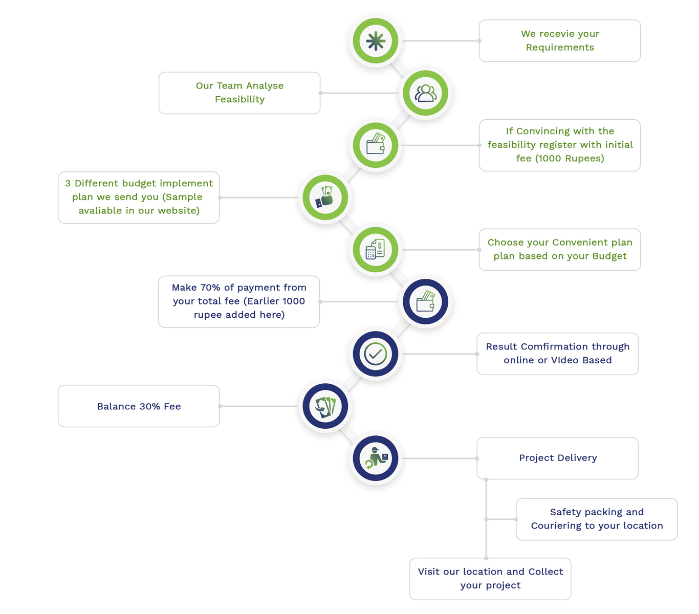
Simulation Projects Workflow
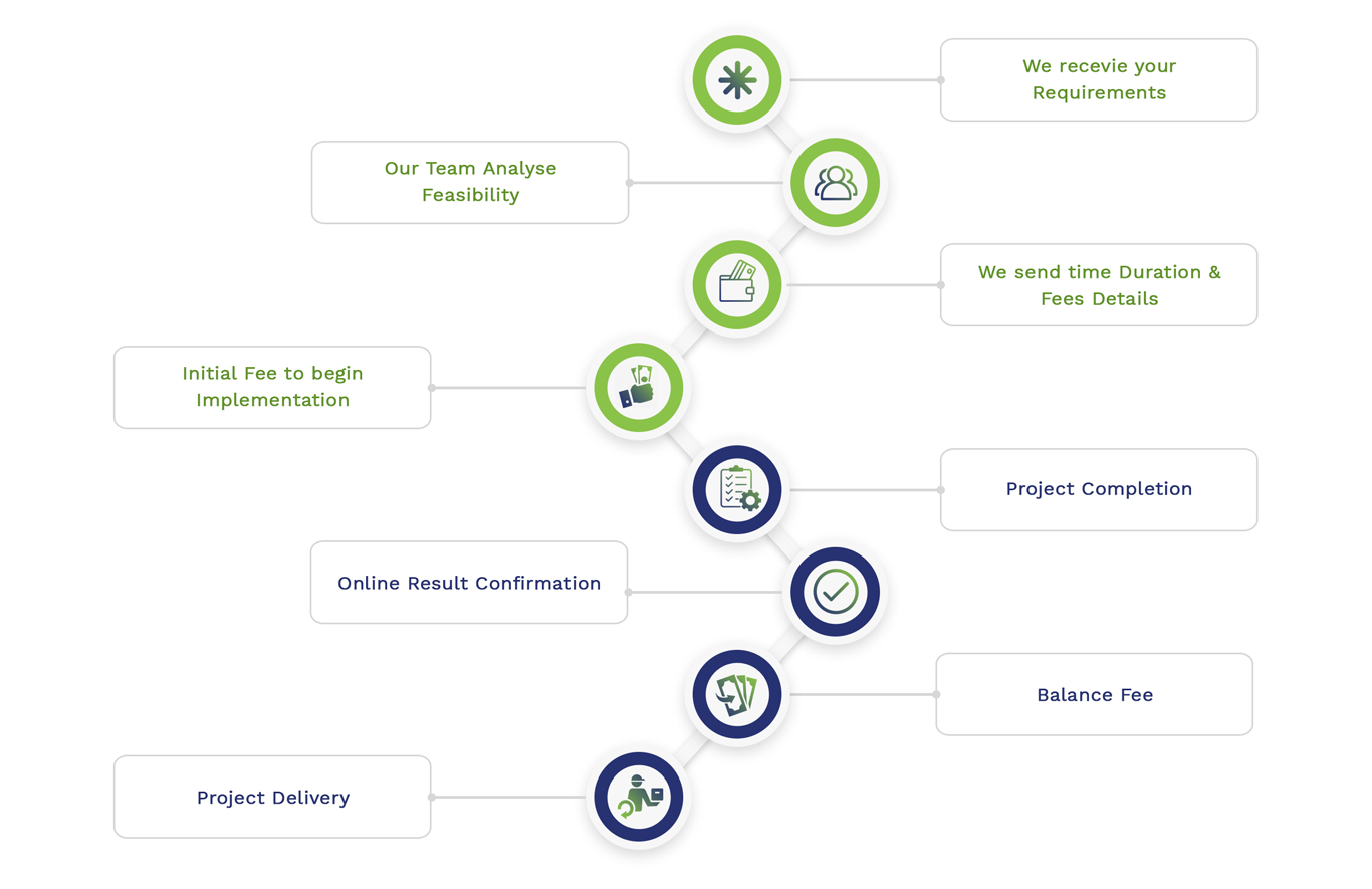
Embedded Projects Workflow