 Matlab
 Simulink
 NS3
NS3 OMNET++
 COOJA
COOJA CONTIKI OS
 NS2
NS2
Instant MATLAB Help are provided by our developers across several research areas, if you want immediate support then drop us all your doubts through our mail id we will give you immediate solution with proper explanation. We work on all areas of MATLAB by giving you best simulation results. MATLAB plays a crucial role in an efficient manner. To carry out a data analysis in MATLAB, we suggest a thorough instruction by involving visualization, highly innovative approaches like clustering and regression, importing data, and fundamental statistical analysis.
In-depth Instruction to Data Analysis in MATLAB
- Importing Data
From different sources like databases, Excel files, and CSV files, we can load data.
Instance: Importing Data from a CSV File
% Import data from a CSV file
data = readtable(‘your_data.csv’);
% Display the first few rows of the table
head(data);
- Fundamental Statistical Analysis
To acquire an outline of the data, fundamental statistical analysis has to be carried out.
Instance: Descriptive Statistics
% Calculate summary statistics
summaryStats = summary(data);
% Display summary statistics
disp(summaryStats);
% Calculate mean and standard deviation for a specific column
meanValue = mean(data.YourColumnName);
stdValue = std(data.YourColumnName);
fprintf(‘Mean: %.2f, Standard Deviation: %.2f\n’, meanValue, stdValue);
- Data Visualization
In order to interpret the connections and distribution, the data must be visualized with different kinds of plots.
Instance: Histogram and Scatter Plot
% Histogram of a specific column
figure;
histogram(data.YourColumnName);
title(‘Histogram of YourColumnName’);
xlabel(‘Values’);
ylabel(‘Frequency’);
% Scatter plot between two columns
figure;
scatter(data.Column1, data.Column2);
title(‘Scatter Plot of Column1 vs Column2’);
xlabel(‘Column1’);
ylabel(‘Column2’);
- Data Cleaning
Assure that the dataset is prepared for the analysis process by managing anomalies and missing values.
Instance: Handling Missing Data
% Identify missing data
missingData = ismissing(data);
% Display rows with missing data
dataWithMissing = data(any(missingData, 2), :);
disp(dataWithMissing);
% Fill missing data with the mean of the column
dataFilled = fillmissing(data, ‘linear’);
- Regression Analysis
As a means to interpret connections among attributes, we have to carry out regression analysis.
Instance: Linear Regression
% Fit a linear regression model
mdl = fitlm(data, ‘YourDependentVariable ~ YourIndependentVariable1 + YourIndependentVariable2’);
% Display the model summary
disp(mdl);
% Plot the regression line
figure;
plot(mdl);
title(‘Linear Regression Model’);
xlabel(‘Predictors’);
ylabel(‘Response’);
- Clustering Analysis
To detect sets and patterns, the data has to be clustered.
Instance: K-Means Clustering
% Standardize the data
standardizedData = zscore(data{:, :});
% Perform K-means clustering
k = 3; % Number of clusters
[idx, C] = kmeans(standardizedData, k);
% Add cluster information to the table
data.Cluster = idx;
% Visualize the clusters
figure;
gscatter(data.YourColumn1, data.YourColumn2, data.Cluster);
title(‘K-Means Clustering’);
xlabel(‘YourColumn1’);
ylabel(‘YourColumn2’);
Complete Instance: Data Analysis Workflow
By integrating the above specified procedures with an example dataset, we provide a complete instance.
% Import data from a CSV file
data = readtable(‘your_data.csv’);
% Display the first few rows of the table
head(data);
% Calculate summary statistics
summaryStats = summary(data);
disp(summaryStats);
% Calculate mean and standard deviation for a specific column
meanValue = mean(data.YourColumnName);
stdValue = std(data.YourColumnName);
fprintf(‘Mean: %.2f, Standard Deviation: %.2f\n’, meanValue, stdValue);
% Histogram of a specific column
figure;
histogram(data.YourColumnName);
title(‘Histogram of YourColumnName’);
xlabel(‘Values’);
ylabel(‘Frequency’);
% Scatter plot between two columns
figure;
scatter(data.Column1, data.Column2);
title(‘Scatter Plot of Column1 vs Column2’);
xlabel(‘Column1’);
ylabel(‘Column2’);
% Identify missing data
missingData = ismissing(data);
% Display rows with missing data
dataWithMissing = data(any(missingData, 2), :);
disp(dataWithMissing);
% Fill missing data with the mean of the column
dataFilled = fillmissing(data, ‘linear’);
% Fit a linear regression model
mdl = fitlm(data, ‘YourDependentVariable ~ YourIndependentVariable1 + YourIndependentVariable2’);
disp(mdl);
% Plot the regression line
figure;
plot(mdl);
title(‘Linear Regression Model’);
xlabel(‘Predictors’);
ylabel(‘Response’);
% Standardize the data
standardizedData = zscore(data{:, :});
% Perform K-means clustering
k = 3; % Number of clusters
[idx, C] = kmeans(standardizedData, k);
% Add cluster information to the table
data.Cluster = idx;
% Visualize the clusters
figure;
gscatter(data.YourColumn1, data.YourColumn2, data.Cluster);
title(‘K-Means Clustering’);
xlabel(‘YourColumn1’);
ylabel(‘YourColumn2’);
Instant matlab help with all research areas
MATLAB is examined as a robust and important platform that is used for various research purposes. For utilizing MATLAB among different research areas such as Image Processing, Optimization, Control Systems, Signal Processing, and Machine Learning, we offer some sample codes and concise overview explicitly.
- Machine Learning
Instance: Training a Decision Tree Classifier
% Load sample data
load fisheriris;
data = meas; % Features
labels = species; % Labels
% Split the data into training and testing sets
cv = cvpartition(labels, ‘HoldOut’, 0.3);
XTrain = data(training(cv), :);
YTrain = labels(training(cv), :);
XTest = data(test(cv), :);
YTest = labels(test(cv), :);
% Train a Decision Tree
treeModel = fitctree(XTrain, YTrain);
% Predict and evaluate the Decision Tree
YPred = predict(treeModel, XTest);
accuracy = sum(YPred == YTest) / numel(YTest);
fprintf(‘Decision Tree Accuracy: %.2f%%\n’, accuracy * 100);
- Signal Processing
Instance: Modeling a Low-Pass FIR Filter
% Design a low-pass FIR filter
fs = 1000; % Sampling frequency
f_cutoff = 150; % Cutoff frequency
n = 50; % Filter order
b = fir1(n, f_cutoff/(fs/2)); % FIR filter coefficients
% Plot the frequency response
freqz(b, 1, 1024, fs);
title(‘Frequency Response of FIR Filter’);
- Control Systems
Instance: PID Controller Design
% Define system parameters
num = [1];
den = [1, 10, 20];
sys = tf(num, den);
% Design PID controller
Kp = 1;
Ki = 1;
Kd = 1;
pid_controller = pid(Kp, Ki, Kd);
% Create closed-loop system
closed_loop_sys = feedback(pid_controller * sys, 1);
% Plot step response
step(closed_loop_sys);
title(‘Step Response with PID Controller’);
- Optimization
Instance: Utilizing Genetic Algorithm for Optimization
% Define the objective function
objective = @(x) x(1)^2 + x(2)^2 + 3;
% Set the number of variables
nvars = 2;
% Set the lower and upper bounds of the variables
lb = [-10, -10];
ub = [10, 10];
% Configure GA options
options = optimoptions(‘ga’, ‘Display’, ‘iter’);
% Run the genetic algorithm
[x, fval] = ga(objective, nvars, [], [], [], [], lb, ub, [], options);
% Display the results
disp([‘Optimal x: ‘, num2str(x)]);
disp([‘Optimal value: ‘, num2str(fval)]);
- Image Processing
Instance: Edge Detection with Canny Approach
% Load an image
img = imread(‘peppers.png’);
grayImg = rgb2gray(img);
% Perform edge detection using Canny method
edges = edge(grayImg, ‘Canny’);
% Display the original image and the edges
figure;
subplot(1, 2, 1);
imshow(grayImg);
title(‘Original Image’);
subplot(1, 2, 2);
imshow(edges);
title(‘Edges Detected using Canny’);
- Deep Learning
Instance: Training a Convolutional Neural Network (CNN) for Image Categorization
% Load sample data
digitDatasetPath = fullfile(matlabroot, ‘toolbox’, ‘nnet’, ‘nndemos’, ‘nndatasets’, ‘DigitDataset’);
imds = imageDatastore(digitDatasetPath, ‘IncludeSubfolders’, true, ‘LabelSource’, ‘foldernames’);
% Split the data into training and testing sets
[imdsTrain, imdsTest] = splitEachLabel(imds, 0.7, ‘randomize’);
% Define the network architecture
layers = [
imageInputLayer([28 28 1])
convolution2dLayer(3, 8, ‘Padding’, ‘same’)
batchNormalizationLayer
reluLayer
maxPooling2dLayer(2, ‘Stride’, 2)
convolution2dLayer(3, 16, ‘Padding’, ‘same’)
batchNormalizationLayer
reluLayer
maxPooling2dLayer(2, ‘Stride’, 2)
convolution2dLayer(3, 32, ‘Padding’, ‘same’)
batchNormalizationLayer
reluLayer
fullyConnectedLayer(10)
softmaxLayer
classificationLayer];
% Set training options
options = trainingOptions(‘sgdm’, ‘MaxEpochs’, 4, ‘ValidationFrequency’, 30, ‘Verbose’, false, ‘Plots’, ‘training-progress’);
% Train the network
net = trainNetwork(imdsTrain, layers, options);
% Evaluate the network
YPred = classify(net, imdsTest);
YTest = imdsTest.Labels;
accuracy = sum(YPred == YTest) / numel(YTest);
fprintf(‘Test Accuracy: %.2f%%\n’, accuracy * 100);
- Financial Data Analysis
Instance: Time Series Prediction with ARIMA
% Load financial data
data = load(‘Data_AAPL.mat’);
prices = data.DataTable.Close;
dates = data.DataTable.Date;
% Convert to time series object
ts = timeseries(prices, dates);
% Plot the data
figure;
plot(ts.Time, ts.Data);
title(‘AAPL Stock Prices’);
xlabel(‘Date’);
ylabel(‘Price’);
% Fit an ARIMA model
model = arima(‘Constant’, 0, ‘D’, 1, ‘Seasonality’, 12, ‘MALags’, 1, ‘SMALags’, 12);
fit = estimate(model, ts.Data);
% Forecast future prices
numPeriods = 12;
[forecast, ~, conf] = forecast(fit, numPeriods, ‘Y0’, ts.Data);
% Plot forecast results
figure;
plot(ts.Time, ts.Data, ‘b’, ‘DisplayName’, ‘Observed’);
hold on;
plot(ts.Time(end) + (1:numPeriods)’, forecast, ‘r’, ‘DisplayName’, ‘Forecast’);
plot(ts.Time(end) + (1:numPeriods)’, conf, ‘k–‘, ‘DisplayName’, ‘Confidence Interval’);
legend;
title(‘AAPL Stock Price Forecast’);
xlabel(‘Date’);
ylabel(‘Price’);
For conducting a data analysis in MATLAB, an in-depth instruction is provided by us, which can assist you in an effective way. In order to employ MATLAB among several research areas, we recommended a few sample codes and brief outlines.
Looking for coding guidance then don’t hesitate to reach us out.
Subscribe Our Youtube Channel
You can Watch all Subjects Matlab & Simulink latest Innovative Project Results

Our services
We want to support Uncompromise Matlab service for all your Requirements Our Reseachers and Technical team keep update the technology for all subjects ,We assure We Meet out Your Needs.
Our Services
- Matlab Research Paper Help
- Matlab assignment help
- Matlab Project Help
- Matlab Homework Help
- Simulink assignment help
- Simulink Project Help
- Simulink Homework Help
- Matlab Research Paper Help
- NS3 Research Paper Help
- Omnet++ Research Paper Help
Our Benefits
- Customised Matlab Assignments
- Global Assignment Knowledge
- Best Assignment Writers
- Certified Matlab Trainers
- Experienced Matlab Developers
- Over 400k+ Satisfied Students
- Ontime support
- Best Price Guarantee
- Plagiarism Free Work
- Correct Citations
Expert Matlab services just 1-click

Delivery Materials
Unlimited support we offer you
For better understanding purpose we provide following Materials for all Kind of Research & Assignment & Homework service.
 Programs
 Designs
 Simulations
 Results
 Graphs
 Result snapshot
 Video Tutorial
 Instructions Profile
  Sofware Install Guide
 Execution Guidance
  Explanations
 Implement Plan
Matlab Projects
Matlab projects innovators has laid our steps in all dimension related to math works.Our concern support matlab projects for more than 10 years.Many Research scholars are benefited by our matlab projects service.We are trusted institution who supplies matlab projects for many universities and colleges.
Reasons to choose Matlab Projects .org???
Our Service are widely utilized by Research centers.More than 5000+ Projects & Thesis has been provided by us to Students & Research Scholars. All current mathworks software versions are being updated by us.
Our concern has provided the required solution for all the above mention technical problems required by clients with best Customer Support.
- Novel Idea
- Ontime Delivery
- Best Prices
- Unique Work
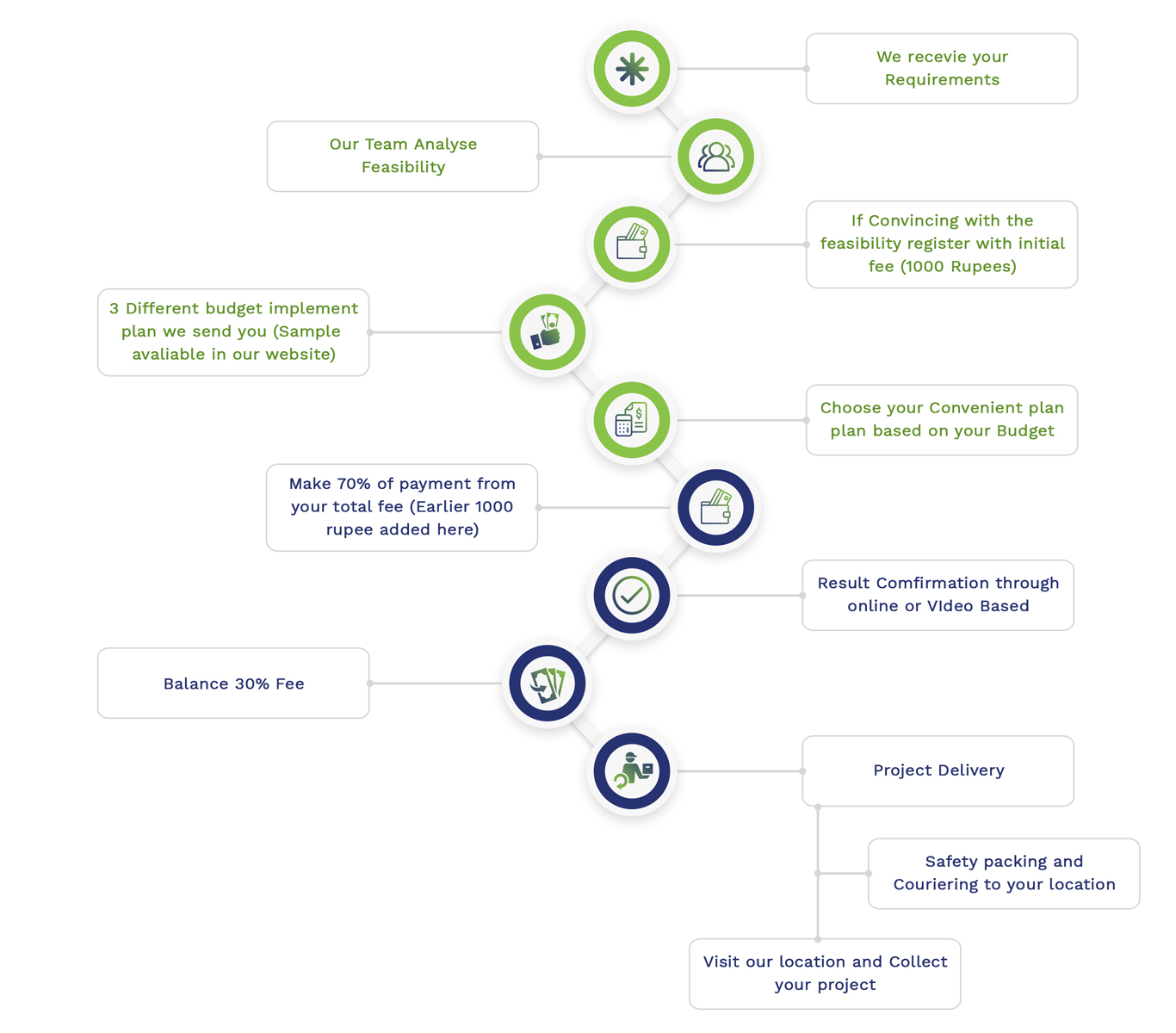
Simulation Projects Workflow
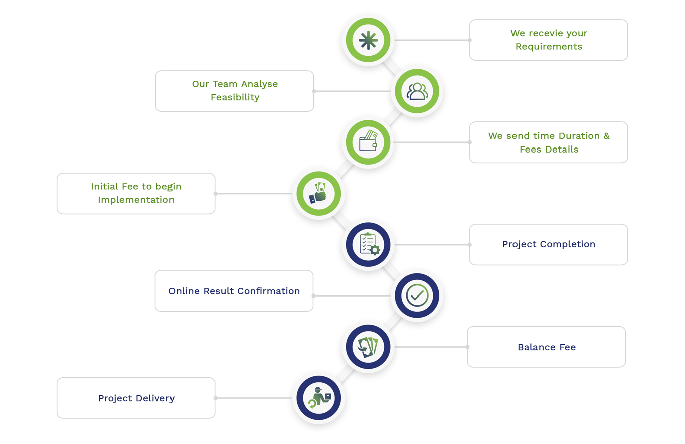
Embedded Projects Workflow