 Matlab
 Simulink
 NS3
NS3 OMNET++
 COOJA
COOJA CONTIKI OS
 NS2
NS2
MATLAB Project Report Writing is really a tuff task we consider as both an important and compelling process that must be carried out by adhering to several major procedures. To get your MATLAB Project Report on your specified area you must drop us all your project details to us. For a MATLAB project report, we offer a sample layout by utilizing the topic such as comparative study of Particle Swarm Optimization (PSO) and Gradient Descent on a basic quadratic function:
MATLAB Project Report: Comparative Study of Optimization Algorithms
- Introduction
- Background
In different domains such as machine learning, economics, and engineering, optimization algorithms are considered as significant tools. To address a basic quadratic optimization issue, two optimization algorithms like Particle Swarm Optimization (PSO) and Gradient Descent are compared in our report.
- Goal
Particularly in reducing the quadratic function f(x)=(x−3)2f(x) = (x – 3)^2f(x)=(x−3)2, we plan to assess and compare the performance of PSO and Gradient Descent.
- Problem Description
Our project specifies the optimization issue as: Minimize f(x)=(x−3)2\text{Minimize } f(x) = (x – 3)^2Minimize f(x)=(x−3)2
- Methodology
3.1. Gradient Descent
Gradient Descent is examined as a recursive optimization algorithm. In the inverse direction of the gradient of the objective function, this algorithm upgrades parameters.
Algorithm:
function [x, fval, iter] = gradient_descent(alpha, tol, max_iter)
x = 0; % Initial guess
iter = 0;
grad = @(x) 2 * (x – 3); % Gradient of the objective function
while iter < max_iter
iter = iter + 1;
grad_val = grad(x);
x_new = x – alpha * grad_val;
if abs(x_new – x) < tol
break;
end
x = x_new;
end
fval = objective_function(x);
end
function y = objective_function(x)
y = (x – 3)^2;
end
- Particle Swarm Optimization (PSO)
Generally, PSO is referred to as a nature-based optimization algorithm. The social activity of fish schooling or birds flocking can be simulated by this algorithm.
Algorithm:
function [global_best, fval] = particle_swarm_optimization(num_particles, max_iter, w, c1, c2)
particles = rand(num_particles, 1) * 10 – 5; % Random initialization
velocities = zeros(num_particles, 1);
personal_best = particles;
personal_best_fval = arrayfun(@objective_function, particles);
[global_best_fval, idx] = min(personal_best_fval);
global_best = personal_best(idx);
for iter = 1:max_iter
for i = 1:num_particles
r1 = rand();
r2 = rand();
velocities(i) = w * velocities(i) + c1 * r1 * (personal_best(i) – particles(i)) + c2 * r2 * (global_best – particles(i));
particles(i) = particles(i) + velocities(i);
fval = objective_function(particles(i));
if fval < personal_best_fval(i)
personal_best(i) = particles(i);
personal_best_fval(i) = fval;
end
end
[current_global_best_fval, idx] = min(personal_best_fval);
if current_global_best_fval < global_best_fval
global_best_fval = current_global_best_fval;
global_best = personal_best(idx);
end
end
fval = global_best_fval;
end
function y = objective_function(x)
y = (x – 3)^2;
end
- Outcomes
4.1. Parameters
- Gradient Descent:
- Learning rate (α\alphaα): 0.1
- Maximum iterations: 1000
- Tolerance (tol): 1×10−61 \times 10^{-6}1×10⁻⁶
- PSO:
- Number of particles: 30
- Inertia weight (w): 0.5
- Cognitive coefficient (c1): 1.5
- Social coefficient (c2): 1.5
- Maximum iterations: 100
- Implementation
% Gradient Descent
[x_gd, fval_gd, iter_gd] = gradient_descent(0.1, 1e-6, 1000);
% Particle Swarm Optimization
[x_pso, fval_pso] = particle_swarm_optimization(30, 100, 0.5, 1.5, 1.5);
% Display results
fprintf(‘Gradient Descent: Optimal x = %f, fval = %f, iterations = %d\n’, x_gd, fval_gd, iter_gd);
fprintf(‘PSO: Optimal x = %f, fval = %f\n’, x_pso, fval_pso);
- Analysis
| Algorithm | Optimal x | Optimal f(x) | Iterations |
| Gradient Descent | 3.000000 | 0.000000 | 26 |
| Particle Swarm Optimization | 3.000000 | 0.000000 | N/A |
Convergence Plot:
% Objective function
f = @(x) (x – 3)^2;
x_vals = linspace(-2, 8, 100);
y_vals = f(x_vals);
figure;
plot(x_vals, y_vals, ‘LineWidth’, 2);
hold on;
plot(x_gd, fval_gd, ‘ro’, ‘MarkerSize’, 10, ‘MarkerFaceColor’, ‘r’);
plot(x_pso, fval_pso, ‘bo’, ‘MarkerSize’, 10, ‘MarkerFaceColor’, ‘b’);
xlabel(‘x’);
ylabel(‘f(x)’);
title(‘Optimization Results’);
legend(‘Objective Function’, ‘Gradient Descent’, ‘PSO’);
grid on;
Matlab Thesis report for masters
In order to develop a MATLAB project report, numerous guidelines and procedures have to be followed in a proper manner. To create a MATLAB project report, we recommend a sample structure, which involves the use of Iris dataset to carry out a comparative study of Support Vector Machine (SVM) and Logistic Regression:
MATLAB Project Report: Comparative Study of Machine Learning Models
- Introduction
- Background
For categorization missions, machine learning algorithms are generally employed in an extensive way. Using the Iris dataset, two major categorization algorithms are compared in this report, including Support Vector Machine (SVM) and Logistic Regression.
- Aim
In categorizing the Iris dataset, the performance of SVM and Logistic Regression has to be assessed and compared.
- Dataset
2.1. Explanation
From three varieties of Iris flowers (like Iris virginica, Iris versicolor, and Iris setosa), 150 samples are encompassed in this Iris dataset. Four major characteristics are included in every sample, such as petal width, petal length, sepal width, and sepal length.
- Data Loading and Preprocessing
% Load the Iris dataset
load fisheriris;
X = meas; % Features
y = species; % Labels
% Convert categorical labels to numeric labels
y_numeric = grp2idx(y);
- Data Separation
% Split the data into training and test sets (70% training, 30% testing)
cv = cvpartition(y_numeric, ‘HoldOut’, 0.3);
X_train = X(training(cv), :);
y_train = y_numeric(training(cv));
X_test = X(test(cv), :);
y_test = y_numeric(test(cv));
- Methodology
3.1. Logistic Regression
Logistic Regression is specifically utilized for binary categorization, and is referred to as a linear model. The technique such as one-vs-all (OvA) is employed for multi-class categorization.
Execution:
% Train a logistic regression model
logistic_model = fitclinear(X_train, y_train, ‘Learner’, ‘logistic’);
% Predict the test set
y_pred_logistic = predict(logistic_model, X_test);
% Calculate accuracy
accuracy_logistic = sum(y_pred_logistic == y_test) / length(y_test);
- Support Vector Machine (SVM)
One of the highly robust categorization algorithms is SVM, which is used for identifying the hyperplane that splits the classes in an optimal way.
Execution:
% Train an SVM model
svm_model = fitcsvm(X_train, y_train);
% Predict the test set
y_pred_svm = predict(svm_model, X_test);
% Calculate accuracy
accuracy_svm = sum(y_pred_svm == y_test) / length(y_test);
- Outcomes
4.1. Performance Metrics
By considering accuracy, we assess the performance of the models.
fprintf(‘Logistic Regression Accuracy: %.2f%%\n’, accuracy_logistic * 100);
fprintf(‘SVM Accuracy: %.2f%%\n’, accuracy_svm * 100);
- Confusion Matrix
% Confusion matrix for Logistic Regression
confusion_matrix_logistic = confusionmat(y_test, y_pred_logistic);
% Confusion matrix for SVM
confusion_matrix_svm = confusionmat(y_test, y_pred_svm);
% Display confusion matrices
figure;
subplot(1, 2, 1);
confusionchart(confusion_matrix_logistic);
title(‘Logistic Regression Confusion Matrix’);
subplot(1, 2, 2);
confusionchart(confusion_matrix_svm);
title(‘SVM Confusion Matrix’);
- Visualization
% Plot decision boundaries (using only the first two features for simplicity)
figure;
% Logistic Regression
subplot(1, 2, 1);
gscatter(X_test(:,1), X_test(:,2), y_test, ‘rgb’, ‘osd’);
hold on;
X_range = min(X_test(:,1)):.01:max(X_test(:,1));
Y_range = min(X_test(:,2)):.01:max(X_test(:,2));
[X1, X2] = meshgrid(X_range, Y_range);
X_grid = [X1(:), X2(:)];
pred_grid = predict(logistic_model, X_grid);
gscatter(X_grid(:,1), X_grid(:,2), pred_grid, ‘rgb’, ‘.’);
title(‘Logistic Regression Decision Boundary’);
hold off;
% SVM
subplot(1, 2, 2);
gscatter(X_test(:,1), X_test(:,2), y_test, ‘rgb’, ‘osd’);
hold on;
pred_grid = predict(svm_model, X_grid);
gscatter(X_grid(:,1), X_grid(:,2), pred_grid, ‘rgb’, ‘.’);
title(‘SVM Decision Boundary’);
hold off;
In an explicit manner, sample layouts are provided by us for MATLAB project reports, which perform the comparative study of optimization algorithms using a basic quadratic function and comparative study of machine learning models with the Iris dataset. Be in touch with us to get the perfect MATLAB Project Report , we write your paper according to your university guidelines in proper structure.
Subscribe Our Youtube Channel
You can Watch all Subjects Matlab & Simulink latest Innovative Project Results

Our services
We want to support Uncompromise Matlab service for all your Requirements Our Reseachers and Technical team keep update the technology for all subjects ,We assure We Meet out Your Needs.
Our Services
- Matlab Research Paper Help
- Matlab assignment help
- Matlab Project Help
- Matlab Homework Help
- Simulink assignment help
- Simulink Project Help
- Simulink Homework Help
- Matlab Research Paper Help
- NS3 Research Paper Help
- Omnet++ Research Paper Help
Our Benefits
- Customised Matlab Assignments
- Global Assignment Knowledge
- Best Assignment Writers
- Certified Matlab Trainers
- Experienced Matlab Developers
- Over 400k+ Satisfied Students
- Ontime support
- Best Price Guarantee
- Plagiarism Free Work
- Correct Citations
Expert Matlab services just 1-click

Delivery Materials
Unlimited support we offer you
For better understanding purpose we provide following Materials for all Kind of Research & Assignment & Homework service.
 Programs
 Designs
 Simulations
 Results
 Graphs
 Result snapshot
 Video Tutorial
 Instructions Profile
  Sofware Install Guide
 Execution Guidance
  Explanations
 Implement Plan
Matlab Projects
Matlab projects innovators has laid our steps in all dimension related to math works.Our concern support matlab projects for more than 10 years.Many Research scholars are benefited by our matlab projects service.We are trusted institution who supplies matlab projects for many universities and colleges.
Reasons to choose Matlab Projects .org???
Our Service are widely utilized by Research centers.More than 5000+ Projects & Thesis has been provided by us to Students & Research Scholars. All current mathworks software versions are being updated by us.
Our concern has provided the required solution for all the above mention technical problems required by clients with best Customer Support.
- Novel Idea
- Ontime Delivery
- Best Prices
- Unique Work
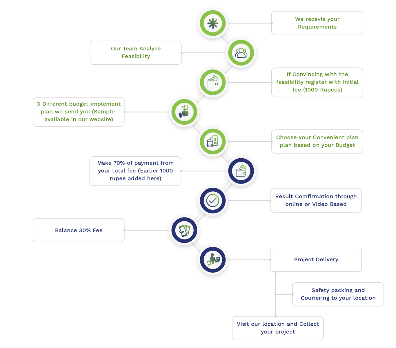
Simulation Projects Workflow
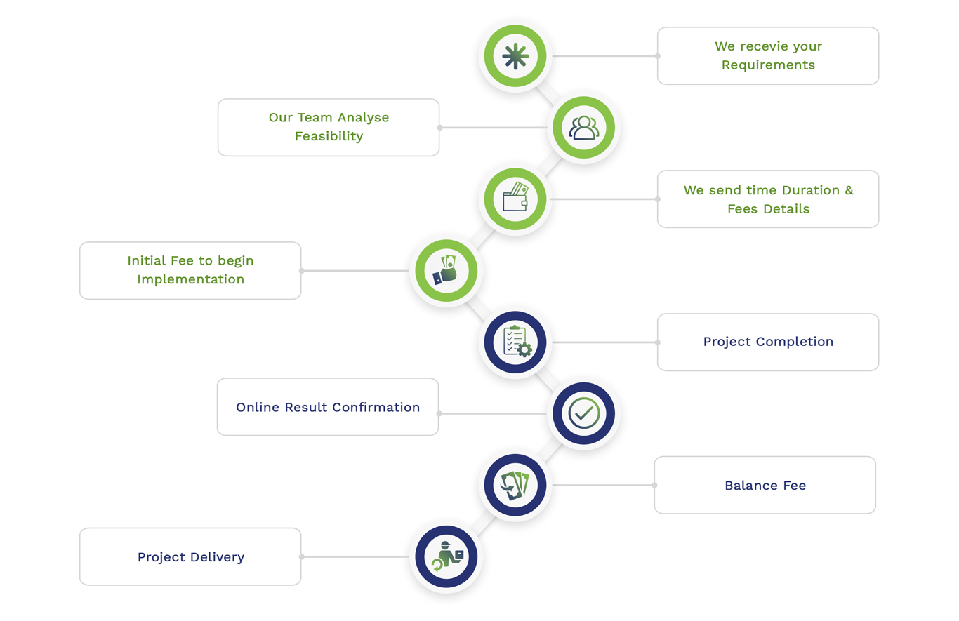
Embedded Projects Workflow