 Matlab
 Simulink
 NS3
NS3 OMNET++
 COOJA
COOJA CONTIKI OS
 NS2
NS2
MATLAB Experts Online are given by us with detailed implementation and explanation. If you are struggling in any area of MATLAB then be in touch with us to get good solution. By online itself you can get best results for all types of MATLAB issues. In recent years, several project ideas have evolved based on the simulation of various protocols. By considering different protocol simulations, we suggest a few significant instances that might be more intriguing to you:
Sample 1: Simulating a Basic MAC Protocol
Goal
For a wireless network, a basic Medium Access Control (MAC) protocol has to be simulated, in which nodes compete to gain access to a distributed channel.
MATLAB Code
% Simulation parameters
numNodes = 10;
numSlots = 1000;
probabilityTransmit = 0.1;
% Initialize variables
channelState = zeros(1, numSlots);
transmissions = zeros(numNodes, numSlots);
% Simulate the MAC protocol
for slot = 1:numSlots
for node = 1:numNodes
if rand < probabilityTransmit
transmissions(node, slot) = 1;
end
end
% Check for collisions
if sum(transmissions(:, slot)) > 1
channelState(slot) = -1; % Collision
elseif sum(transmissions(:, slot)) == 1
channelState(slot) = find(transmissions(:, slot)); % Successful transmission
else
channelState(slot) = 0; % Idle
end
end
% Analyze results
numCollisions = sum(channelState == -1);
numSuccesses = sum(channelState > 0);
numIdle = sum(channelState == 0);
% Display results
disp([‘Number of Collisions: ‘, num2str(numCollisions)]);
disp([‘Number of Successful Transmissions: ‘, num2str(numSuccesses)]);
disp([‘Number of Idle Slots: ‘, num2str(numIdle)]);
Sample 2: Simulating the ALOHA Protocol
Goal
The ALOHA protocol must be simulated, in which collisions can arise through nodes that transmit packets in a random way.
MATLAB Code
% Simulation parameters
numNodes = 10;
numSlots = 1000;
probabilityTransmit = 0.1;
% Initialize variables
channelState = zeros(1, numSlots);
transmissions = zeros(numNodes, numSlots);
% Simulate the ALOHA protocol
for slot = 1:numSlots
for node = 1:numNodes
if rand < probabilityTransmit
transmissions(node, slot) = 1;
end
end
% Check for collisions
if sum(transmissions(:, slot)) > 1
channelState(slot) = -1; % Collision
elseif sum(transmissions(:, slot)) == 1
channelState(slot) = find(transmissions(:, slot)); % Successful transmission
else
channelState(slot) = 0; % Idle
end
end
% Analyze results
numCollisions = sum(channelState == -1);
numSuccesses = sum(channelState > 0);
numIdle = sum(channelState == 0);
% Display results
disp([‘Number of Collisions: ‘, num2str(numCollisions)]);
disp([‘Number of Successful Transmissions: ‘, num2str(numSuccesses)]);
disp([‘Number of Idle Slots: ‘, num2str(numIdle)]);
Sample 3: Simulating the CSMA/CD Protocol
Goal
In this project, we focus on simulating the CSMA/CD protocol (Carrier Sense Multiple Access with Collision Detection).
MATLAB Code
% Simulation parameters
numNodes = 10;
numSlots = 1000;
probabilityTransmit = 0.1;
% Initialize variables
channelState = zeros(1, numSlots);
transmissions = zeros(numNodes, numSlots);
backoff = zeros(numNodes, 1);
% Simulate the CSMA/CD protocol
for slot = 1:numSlots
for node = 1:numNodes
if backoff(node) > 0
backoff(node) = backoff(node) – 1;
elseif rand < probabilityTransmit
transmissions(node, slot) = 1;
end
end
% Check for collisions
if sum(transmissions(:, slot)) > 1
channelState(slot) = -1; % Collision
% Random backoff for nodes involved in collision
collidingNodes = find(transmissions(:, slot));
backoff(collidingNodes) = randi([1, 10], length(collidingNodes), 1);
elseif sum(transmissions(:, slot)) == 1
channelState(slot) = find(transmissions(:, slot)); % Successful transmission
else
channelState(slot) = 0; % Idle
end
end
% Analyze results
numCollisions = sum(channelState == -1);
numSuccesses = sum(channelState > 0);
numIdle = sum(channelState == 0);
% Display results
disp([‘Number of Collisions: ‘, num2str(numCollisions)]);
disp([‘Number of Successful Transmissions: ‘, num2str(numSuccesses)]);
disp([‘Number of Idle Slots: ‘, num2str(numIdle)]);
Sample 4: Simulating the LoRaWAN Protocol
Goal
By concentrating on data sharing from end devices to a gateway, the LoRaWAN protocol should be simulated.
MATLAB Code
% Simulation parameters
numDevices = 50;
numSlots = 1000;
probabilityTransmit = 0.01;
spreadingFactor = 7;
% Initialize variables
channelState = zeros(1, numSlots);
transmissions = zeros(numDevices, numSlots);
receivedPackets = 0;
% Simulate LoRaWAN protocol
for slot = 1:numSlots
for device = 1:numDevices
if rand < probabilityTransmit
transmissions(device, slot) = 1;
end
end
% Check for collisions
if sum(transmissions(:, slot)) > 1
channelState(slot) = -1; % Collision
elseif sum(transmissions(:, slot)) == 1
channelState(slot) = find(transmissions(:, slot)); % Successful transmission
receivedPackets = receivedPackets + 1;
else
channelState(slot) = 0; % Idle
end
end
% Analyze results
numCollisions = sum(channelState == -1);
numIdle = sum(channelState == 0);
% Display results
disp([‘Number of Collisions: ‘, num2str(numCollisions)]);
disp([‘Number of Successful Packets: ‘, num2str(receivedPackets)]);
disp([‘Number of Idle Slots: ‘, num2str(numIdle)]);
Sample 5: Simulating TCP/IP Protocol
Goal
In order to interpret the congestion control and flow control techniques, we simulate a basic TCP/IP protocol.
MATLAB Code
% Simulation parameters
numPackets = 100;
packetLossProbability = 0.1;
RTT = 100; % Round-Trip Time in ms
cwnd = 1; % Initial congestion window size
ssthresh = 64; % Slow start threshold
% Initialize variables
packetsSent = 0;
packetsAcknowledged = 0;
packetsLost = 0;
time = 0;
% Simulate TCP/IP protocol
while packetsAcknowledged < numPackets
for i = 1:cwnd
if packetsSent < numPackets
packetsSent = packetsSent + 1;
if rand < packetLossProbability
packetsLost = packetsLost + 1;
else
packetsAcknowledged = packetsAcknowledged + 1;
end
end
end
% Update congestion window size
if packetsLost > 0
ssthresh = max(cwnd / 2, 1);
cwnd = 1;
packetsLost = 0;
else
if cwnd < ssthresh
cwnd = cwnd * 2; % Exponential growth (slow start)
else
cwnd = cwnd + 1; % Linear growth (congestion avoidance)
end
end
% Increment time by RTT
time = time + RTT;
end
% Display results
disp([‘Total Packets Sent: ‘, num2str(packetsSent)]);
disp([‘Total Packets Acknowledged: ‘, num2str(packetsAcknowledged)]);
disp([‘Total Simulation Time: ‘, num2str(time), ‘ ms’]);
Matlab experts for all research departments
MATLAB is examined as a robust platform that is generally employed in an extensive manner across numerous fields. For utilization of MATLAB in various domains like Biomedical Engineering, Civil Engineering, Mechanical Engineering, Electrical Engineering, and Computer Science, we list out some interesting topics and suitable instances:
Computer Science and Engineering
Topic: Image Processing and Computer Vision
Instance: Edge Detection with Canny Approach
% Load an image
img = imread(‘peppers.png’);
grayImg = rgb2gray(img);
% Perform edge detection using the Canny method
edges = edge(grayImg, ‘Canny’);
% Display the original image and the edges
figure;
subplot(1, 2, 1);
imshow(grayImg);
title(‘Original Image’);
subplot(1, 2, 2);
imshow(edges);
title(‘Edges Detected using Canny’);
Topic: Machine Learning
Instance: Training a Decision Tree Classifier
% Load sample data
load fisheriris;
data = meas;
labels = species;
% Train a decision tree classifier
tree = fitctree(data, labels);
% View the tree
view(tree, ‘Mode’, ‘graph’);
Electrical and Electronics Engineering
Topic: Signal Processing
Instance: Modeling a Digital Filter
% Design parameters
Fs = 1000; % Sampling frequency
Fp = 200; % Passband frequency
Fst = 250; % Stopband frequency
Ap = 1; % Passband ripple
Ast = 60; % Stopband attenuation
% Design the filter using the Kaiser window method
d = designfilt(‘lowpassfir’, ‘PassbandFrequency’, Fp, ‘StopbandFrequency’, Fst, …
‘PassbandRipple’, Ap, ‘StopbandAttenuation’, Ast, ‘SampleRate’, Fs);
% View the filter response
fvtool(d);
% Apply the filter to a signal
t = 0:1/Fs:1-1/Fs;
x = sin(2*pi*100*t) + 0.5*sin(2*pi*300*t); % Example signal
y = filter(d, x);
% Plot the original and filtered signals
figure;
subplot(2, 1, 1);
plot(t, x);
title(‘Original Signal’);
subplot(2, 1, 2);
plot(t, y);
title(‘Filtered Signal’);
Topic: Control Systems
Instance: PID Controller Design
% Define system parameters
num = [1];
den = [1, 10, 20];
sys = tf(num, den);
% Design a PID controller
Kp = 1;
Ki = 1;
Kd = 1;
pid_controller = pid(Kp, Ki, Kd);
% Create closed-loop system
cl_sys = feedback(pid_controller * sys, 1);
% Simulate step response
figure;
step(cl_sys);
title(‘Step Response with PID Controller’);
Mechanical Engineering
Topic: Finite Element Analysis (FEA)
Instance: Structural Analysis of a Cantilever Beam
% Define beam parameters
L = 2; % Length of the beam
E = 210e9; % Young’s modulus (Pa)
I = 1e-4; % Moment of inertia (m^4)
q = 1000; % Uniform load (N/m)
% Number of elements and nodes
n_elements = 10;
n_nodes = n_elements + 1;
% Element length
le = L / n_elements;
% Stiffness matrix assembly
K = zeros(n_nodes);
F = zeros(n_nodes, 1);
for i = 1:n_elements
ke = E*I/le^3 * [12 6*le -12 6*le; 6*le 4*le^2 -6*le 2*le^2; -12 -6*le 12 -6*le; 6*le 2*le^2 -6*le 4*le^2];
K(i:i+3, i:i+3) = K(i:i+3, i:i+3) + ke;
fe = q*le/2 * [1; le/6; 1; -le/6];
F(i:i+1) = F(i:i+1) + fe(1:2);
end
% Apply boundary conditions
K_reduced = K(2:end, 2:end);
F_reduced = F(2:end);
% Solve for displacements
U = K_reduced \ F_reduced;
U = [0; U]; % Add zero displacement at the fixed end
% Plot deflection
x = linspace(0, L, n_nodes);
plot(x, U);
title(‘Beam Deflection’);
xlabel(‘Length (m)’);
ylabel(‘Deflection (m)’);
Civil Engineering
Topic: Structural Dynamics
Instance: Vibration Analysis of a Multi-Story Building
% Define system parameters
m = 1; % Mass (kg)
k = 100; % Stiffness (N/m)
damping_ratio = 0.05;
% Number of stories
n_stories = 3;
% Mass and stiffness matrices
M = m * eye(n_stories);
K = k * (diag(2*ones(n_stories, 1)) – diag(ones(n_stories-1, 1), 1) – diag(ones(n_stories-1, 1), -1));
% Damping matrix
C = damping_ratio * (M + K);
% Solve the eigenvalue problem
[V, D] = eig(K, M);
% Natural frequencies (rad/s)
wn = sqrt(diag(D));
% Plot mode shapes
figure;
for i = 1:n_stories
subplot(n_stories, 1, i);
plot(1:n_stories, V(:,i));
title([‘Mode Shape ‘, num2str(i)]);
xlabel(‘Story’);
ylabel(‘Amplitude’);
end
Biomedical Engineering
Topic: Biomedical Signal Processing
Instance: ECG Signal Denoising
% Load ECG signal
load(‘ecgSignal.mat’); % Assume ecgSignal contains ECG data
fs = 500; % Sampling frequency
% Design a low-pass filter
fcut = 50; % Cutoff frequency (Hz)
[b, a] = butter(4, fcut/(fs/2), ‘low’);
% Filter the ECG signal
ecgFiltered = filtfilt(b, a, ecgSignal);
% Plot original and filtered ECG signals
t = (0:length(ecgSignal)-1) / fs;
figure;
subplot(2, 1, 1);
plot(t, ecgSignal);
title(‘Original ECG Signal’);
xlabel(‘Time (s)’);
ylabel(‘Amplitude’);
subplot(2, 1, 2);
plot(t, ecgFiltered);
title(‘Filtered ECG Signal’);
xlabel(‘Time (s)’);
ylabel(‘Amplitude’);
On the basis of the protocol simulations, we recommended several major instances, along with explicit goals and MATLAB codes. As a means to utilize MATLAB in various domains, numerous fascinating topics and appropriate instances are proposed by us in a clear way. We have the best team to guide in MATLAB by our Experts in Online who gives immediate response within 30minutes.Drop us with all your details our help desk with give you proper results.
Subscribe Our Youtube Channel
You can Watch all Subjects Matlab & Simulink latest Innovative Project Results

Our services
We want to support Uncompromise Matlab service for all your Requirements Our Reseachers and Technical team keep update the technology for all subjects ,We assure We Meet out Your Needs.
Our Services
- Matlab Research Paper Help
- Matlab assignment help
- Matlab Project Help
- Matlab Homework Help
- Simulink assignment help
- Simulink Project Help
- Simulink Homework Help
- Matlab Research Paper Help
- NS3 Research Paper Help
- Omnet++ Research Paper Help
Our Benefits
- Customised Matlab Assignments
- Global Assignment Knowledge
- Best Assignment Writers
- Certified Matlab Trainers
- Experienced Matlab Developers
- Over 400k+ Satisfied Students
- Ontime support
- Best Price Guarantee
- Plagiarism Free Work
- Correct Citations
Expert Matlab services just 1-click

Delivery Materials
Unlimited support we offer you
For better understanding purpose we provide following Materials for all Kind of Research & Assignment & Homework service.
 Programs
 Designs
 Simulations
 Results
 Graphs
 Result snapshot
 Video Tutorial
 Instructions Profile
  Sofware Install Guide
 Execution Guidance
  Explanations
 Implement Plan
Matlab Projects
Matlab projects innovators has laid our steps in all dimension related to math works.Our concern support matlab projects for more than 10 years.Many Research scholars are benefited by our matlab projects service.We are trusted institution who supplies matlab projects for many universities and colleges.
Reasons to choose Matlab Projects .org???
Our Service are widely utilized by Research centers.More than 5000+ Projects & Thesis has been provided by us to Students & Research Scholars. All current mathworks software versions are being updated by us.
Our concern has provided the required solution for all the above mention technical problems required by clients with best Customer Support.
- Novel Idea
- Ontime Delivery
- Best Prices
- Unique Work
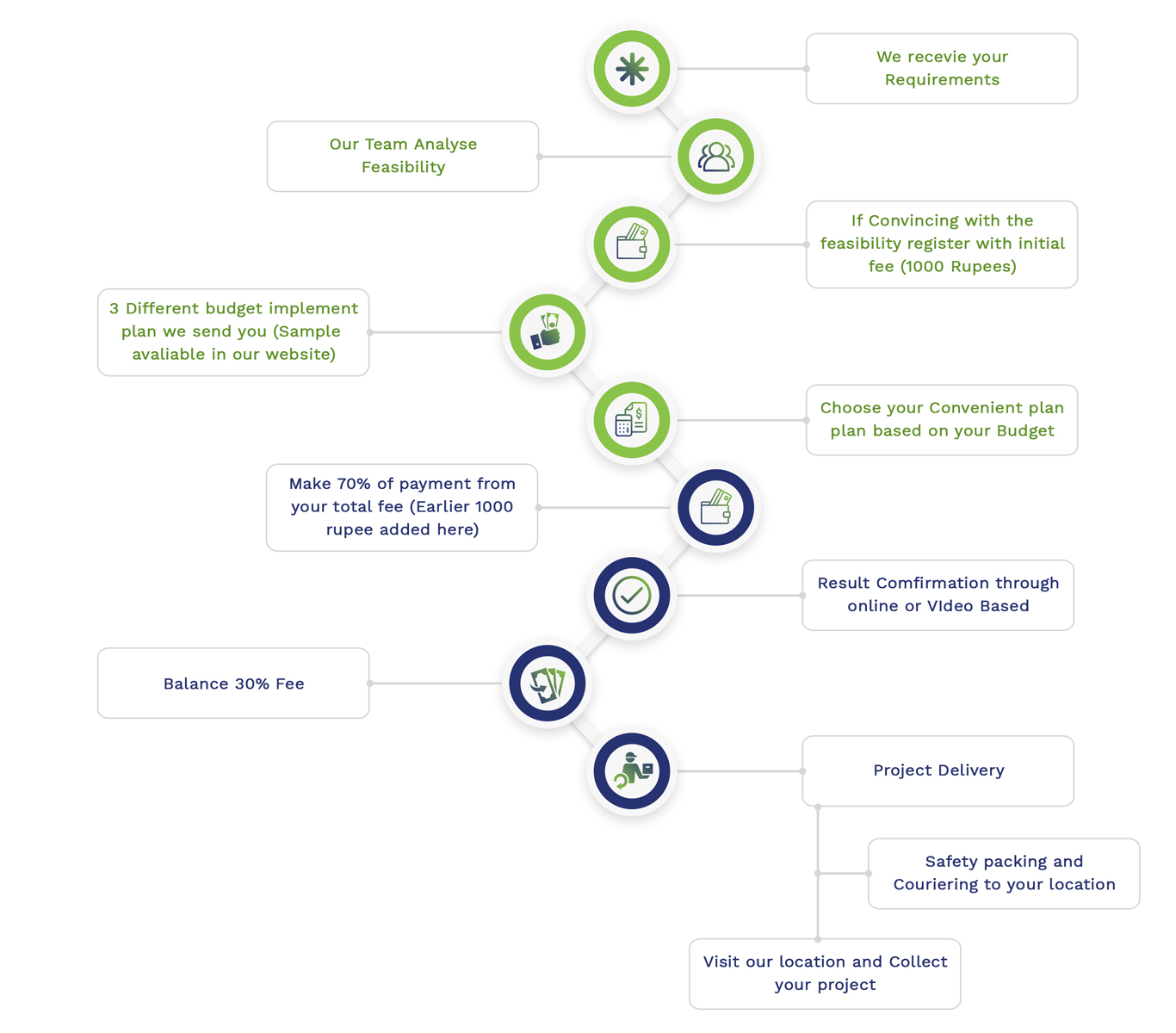
Simulation Projects Workflow
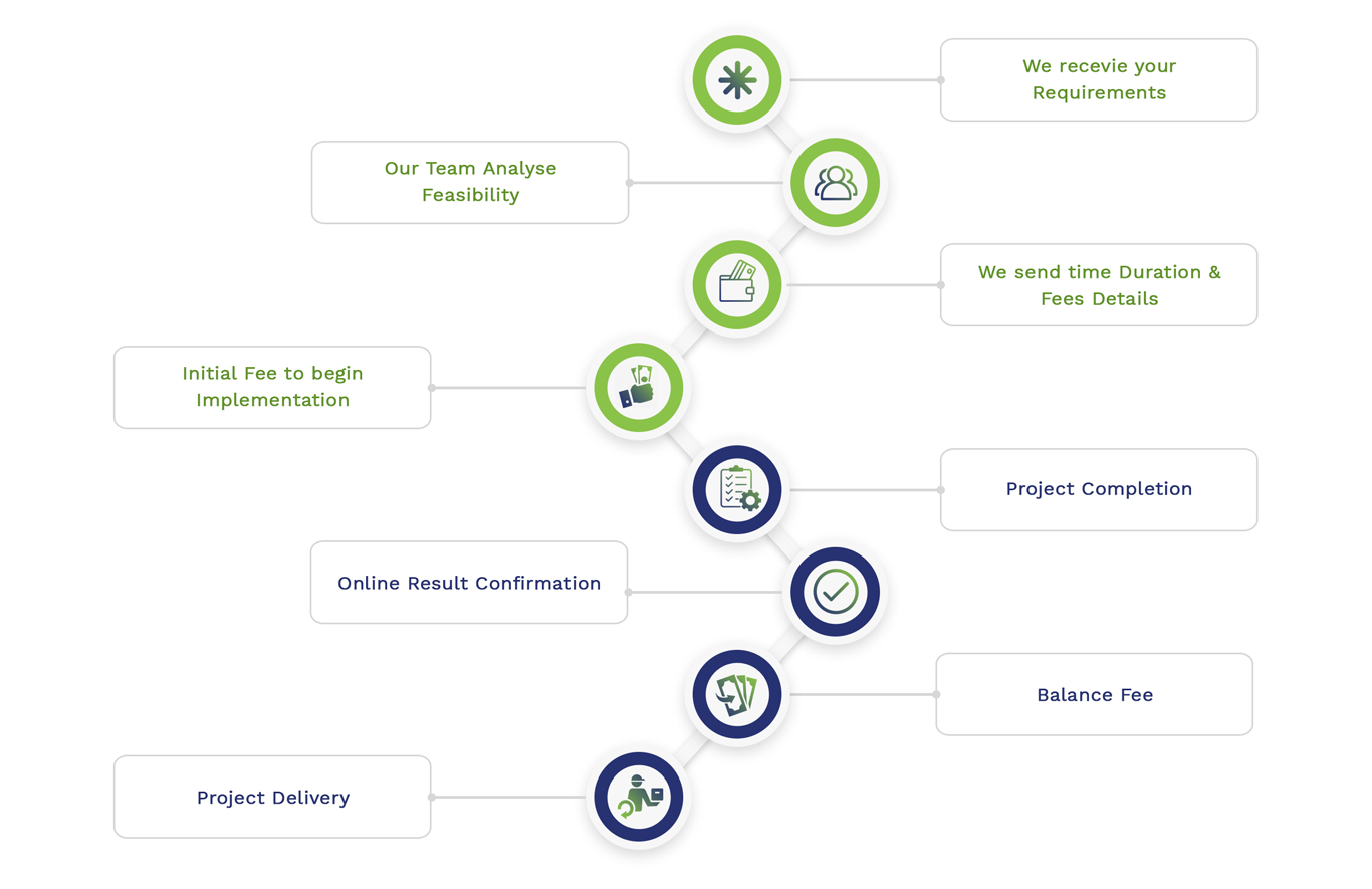
Embedded Projects Workflow