 Matlab
 Simulink
 NS3
NS3 OMNET++
 COOJA
COOJA CONTIKI OS
 NS2
NS2
Optimization Algorithms in MATLAB we at matlabprojects.org employ optimization methods. We have all the leading tools and developers to carry out your simulation and algorithm in an effective way. Just share with us all your reasech details we will provide you with good outcomes by following the protocols. Together with the concise explanations for every topic, we provide 20 significant MATLAB project topics concentrated on optimization methods:
- Genetic Algorithm for Function Optimization
- Explanation: Through the utilization of genetic algorithms, we strengthen a nonlinear function.
- Instance: As a means to identify the global minimum of a complicated function, it is beneficial to employ a genetic algorithm.
% Genetic Algorithm for Function Optimization
fun = @(x) (x(1)-2)^2 + (x(2)-3)^2;
options = optimoptions(‘ga’, ‘Display’, ‘iter’);
[x, fval] = ga(fun, 2, [], [], [], [], [], [], [], options);
disp([‘Optimal solution: ‘, num2str(x)]);
- Particle Swarm Optimization for Clustering
- Explanation: By employing particle swarm optimization, our team intends to group data points.
- Instance: In order to group a collection of 2D data points, focus on utilizing PSO.
% Particle Swarm Optimization for Clustering
data = rand(100, 2); % Random data points
k = 3; % Number of clusters
[idx, centroids] = kmeans(data, k);
- Simulated Annealing for TSP
- Explanation: Generally, the traveling salesman problem has to be addressed through the utilization of simulated annealing.
- Instance: It is approachable to improve the direction for a collection of cities.
% Simulated Annealing for TSP
numberOfCities = 10;
distanceMatrix = rand(numberOfCities);
initialGuess = randperm(numberOfCities);
options = saoptimset(‘PlotFcns’, @saplotbestf);
[x, fval] = simulannealbnd(@tspFun, initialGuess, [], [], options);
disp([‘Optimal route: ‘, num2str(x)]);
- Ant Colony Optimization for Vehicle Routing
- Explanation: By means of employing ant colony optimization, we plan to reinforce vehicle routes.
- Instance: For numerous vehicles, reduce the entire travel distance through the utilization of ACO.
% Ant Colony Optimization for Vehicle Routing
data = [1 2; 3 4; 5 6; 7 8; 9 10];
routes = antColonyOptimization(data, 2); % Assume custom function
disp([‘Optimal routes: ‘, num2str(routes)]);
- Differential Evolution for Portfolio Optimization
- Explanation: Through utilizing differential evolution, our team focuses on enhancing a financial portfolio.
- Instance: At the time of optimizing profits, it is advisable to reduce vulnerabilities.
% Differential Evolution for Portfolio Optimization
fun = @(x) -(x(1)*0.1 + x(2)*0.2 – 0.5*var([x(1)*0.1, x(2)*0.2]));
bounds = [0, 1; 0, 1];
options = optimoptions(‘particleswarm’, ‘Display’, ‘iter’);
[x, fval] = particleswarm(fun, 2, bounds(:,1), bounds(:,2), options);
disp([‘Optimal portfolio: ‘, num2str(x)]);
- Linear Programming for Production Planning
- Explanation: In order to reinforce production plans, we aim to employ linear programming.
- Instance: On resources, focus on enhancing profit provided situations.
% Linear Programming for Production Planning
f = [-5; -4]; % Coefficients for profit
A = [6 4; 1 2; -1 1];
b = [24; 6; 1];
[x, fval] = linprog(f, A, b);
disp([‘Optimal production levels: ‘, num2str(x)]);
- Quadratic Programming for Portfolio Optimization
- Explanation: As a means to strengthen a portfolio, it is beneficial to utilize quadratic programming.
- Instance: Typically, the inconsistency of portfolio profits must be reduced.
% Quadratic Programming for Portfolio Optimization
H = [1 -0.5; -0.5 1];
f = [-2; -3];
A = [];
b = [];
Aeq = [1 1];
beq = [1];
lb = [0; 0];
ub = [];
[x, fval] = quadprog(H, f, A, b, Aeq, beq, lb, ub);
disp([‘Optimal portfolio weights: ‘, num2str(x)]);
- Nonlinear Programming for Mechanical Design
- Explanation: Through the utilization of nonlinear programming, our team plans to improve the model of a mechanical element.
- Instance: In addition to aligning with strength situations, it is better to reduce the weight.
% Nonlinear Programming for Mechanical Design
fun = @(x) x(1)^2 + x(2)^2;
constraints = @(x) deal([], [x(1) + x(2) – 1]);
x0 = [0.5; 0.5];
[x, fval] = fmincon(fun, x0, [], [], [], [], [0; 0], [1; 1], constraints);
disp([‘Optimal design variables: ‘, num2str(x)]);
- Mixed-Integer Programming for Supply Chain Optimization
- Explanation: Generally, supply chain processes have to be enhanced by means of employing mixed-integer programming.
- Instance: In addition to aligning with necessity, decrease the entire expense.
% Mixed-Integer Programming for Supply Chain Optimization
intcon = [1 2];
f = [2 3 4];
A = [1 1 0; 0 1 1];
b = [1; 1];
lb = zeros(1, 3);
ub = [];
[x, fval] = intlinprog(f, intcon, A, b, [], [], lb, ub);
disp([‘Optimal solution: ‘, num2str(x)]);
- Trust-Region Method for Parameter Estimation
- Explanation: By utilizing the trust-region technique, we focus on assessing parameters of a framework.
- Instance: Typically, the parameters of a nonlinear regression framework should be strengthened.
% Trust-Region Method for Parameter Estimation
fun = @(x) sum((y – model(x, t)).^2);
x0 = [1; 1];
options = optimoptions(‘lsqnonlin’, ‘Algorithm’, ‘trust-region-reflective’);
[x, fval] = lsqnonlin(fun, x0, [], [], options);
disp([‘Estimated parameters: ‘, num2str(x)]);
- Interior-Point Method for Network Flow Optimization
- Explanation: Through the utilization of the interior-point technique, our team improves flow of the network.
- Instance: The flow across a network has to be enhanced.
% Interior-Point Method for Network Flow Optimization
fun = @(x) -sum(x);
A = [1 -1 0; 0 1 -1];
b = [0; 0];
x0 = [1; 1; 1];
options = optimoptions(‘fmincon’, ‘Algorithm’, ‘interior-point’);
[x, fval] = fmincon(fun, x0, A, b, [], [], [0; 0; 0], [], [], options);
disp([‘Optimal flow: ‘, num2str(x)]);
- Gradient Descent for Machine Learning
- Explanation: In order to train a machine learning framework, we plan to employ gradient descent.
- Instance: It is appreciable to enhance weights of a linear regression system.
% Gradient Descent for Machine Learning
X = rand(100, 2); % Features
y = rand(100, 1); % Labels
w = zeros(2, 1); % Initial weights
alpha = 0.01; % Learning rate
for i = 1:1000
grad = X’ * (X * w – y) / length(y);
w = w – alpha * grad;
end
disp([‘Optimized weights: ‘, num2str(w’)]);
- Conjugate Gradient for Large-Scale Optimization
- Explanation: By employing the conjugate gradient technique, our team intends to address extensive optimization issues.
- Instance: Focus on reducing a huge quadratic function.
% Conjugate Gradient for Large-Scale Optimization
n = 1000; % Number of variables
A = randn(n); % Random matrix
b = randn(n, 1); % Random vector
x0 = zeros(n, 1); % Initial guess
options = optimoptions(‘fminunc’, ‘Algorithm’, ‘trust-region’, ‘SpecifyObjectiveGradient’, true);
[x, fval] = fminunc(@(x) quadObj(x, A, b), x0, options);
disp([‘Optimized variables: ‘, num2str(x’)]);
function [f, g] = quadObj(x, A, b)
f = 0.5 * x’ * A * x – b’ * x;
g = A * x – b;
end
- Newton’s Method for Optimization
- Explanation: Through the utilization of Newton’s approach, we plan to reinforce functions in an effective manner.
- Instance: The least of a nonlinear function must be identified.
% Newton’s Method for Optimization
fun = @(x) x^2 + sin(x);
grad = @(x) 2*x + cos(x);
hess = @(x) 2 – sin(x);
x = 0; % Initial guess
tol = 1e-6; % Tolerance
for i = 1:100
x_new = x – grad(x)/hess(x);
if abs(x_new – x) < tol
break;
end
x = x_new;
end
disp([‘Optimal solution: ‘, num2str(x)]);
- Lagrange Multipliers for Constrained Optimization
- Explanation: With the aid of Lagrange multipliers, our team aims to address constrained optimization issues.
- Instance: Depending on constraints, it is better to enhance a function.
% Lagrange Multipliers for Constrained Optimization
syms x y lambda
f = x^2 + y^2; % Objective function
g = x + y – 1; % Constraint
L = f + lambda * g;
grad_L = gradient(L, [x, y, lambda]);
sol = solve(grad_L == 0, [x, y, lambda]);
disp([‘Optimal solution: x = ‘, num2str(sol.x), ‘, y = ‘, num2str(sol.y)]);
- Sequential Quadratic Programming for Optimal Control
- Explanation: Generally, control policies have to be strengthened by means of employing sequential quadratic programming.
- Instance: In a vehicle, focus on decreasing fuel utilization.
% Sequential Quadratic Programming for Optimal Control
options = optimoptions(‘fmincon’, ‘Algorithm’, ‘sqp’);
[x, fval] = fmincon(@fuelConsumption, x0, A, b, Aeq, beq, lb, ub, nonlcon, options);
disp([‘Optimal control: ‘, num2str(x’)]);
- Bayesian Optimization for Hyperparameter Tuning
- Explanation: Through the utilization of Bayesian optimization, our team focuses on adjusting hyperparameters of machine learning frameworks.
- Instance: It is advisable to reinforce hyperparameters of an SVM classifier.
% Bayesian Optimization for Hyperparameter Tuning
results = bayesopt(@svmObjective, [optimizableVariable(‘C’, [1e-3, 1e3]), optimizableVariable(‘epsilon’, [0.01, 1])]);
disp([‘Optimal hyperparameters: ‘, results.XAtMinObjective]);
- Augmented Lagrangian Method for Constrained Optimization
- Explanation: With the aid of the augmented Lagrangian approach, we intend to address constrained optimization issues.
- Instance: A function with equality situations must be decreased.
% Augmented Lagrangian Method for Constrained Optimization
fun = @(x) x(1)^2 + x(2)^2;
cons = @(x) x(1) + x(2) – 1;
options = optimoptions(‘fmincon’, ‘Algorithm’, ‘interior-point’, ‘UseParallel’, true);
[x, fval] = fmincon(fun, x0, [], [], [], [], lb, ub, cons, options);
disp([‘Optimal solution: ‘, num2str(x’)]);
- Interior Point Method for Convex Optimization
- Explanation: By employing the interior point approach, our team plans to enhance convex functions.
- Instance: A convex quadratic function has to be reduced.
% Interior Point Method for Convex Optimization
H = [2 0; 0 2];
f = [-2; -2];
A = [1 2; -1 2; 2 1];
b = [2; 2; 3];
options = optimoptions(‘quadprog’, ‘Algorithm’, ‘interior-point-convex’);
[x, fval] = quadprog(H, f, A, b, [], [], [], [], [], options);
disp([‘Optimal solution: ‘, num2str(x’)]);
- Dynamic Programming for Optimal Path Finding
- Explanation: Through the utilization of dynamic programming, we aim to identify the efficient path in a grid.
- Instance: In a 2D grid, focus on decreasing the travel expense.
% Dynamic Programming for Optimal Path Finding
cost = rand(5); % Random cost matrix
n = size(cost, 1);
path = zeros(n);
path(1, 1)
Important 20 optimization algorithms matlab Project Topics
In MATLAB project topics, optimization methods are used for several purposes. Together with short outlines for every topic, we suggest 20 significant optimization method project topics employing MATLAB:
- Gradient Descent Optimization
- Outline: For reducing a function, our team focuses on applying and examining the effectiveness of gradient descent optimization.
- Instance: Through the utilization of gradient descent, it is appreciable to improve a quadratic function.
% Gradient Descent Optimization
f = @(x) x.^2;
df = @(x) 2*x;
x = 10; % Initial guess
alpha = 0.1; % Learning rate
tol = 1e-6; % Tolerance
max_iter = 1000; % Maximum number of iterations
for iter = 1:max_iter
x_new = x – alpha * df(x);
if abs(x_new – x) < tol
break;
end
x = x_new;
end
disp([‘Optimal x: ‘, num2str(x)]);
disp([‘Number of iterations: ‘, num2str(iter)]);
- Newton’s Method Optimization
- Outline: Specifically, for improvement, we plan to implement Newton’s technique and aim to contrast it with other techniques.
- Instance: In order to identify the least of a nonlinear function, focus on employing Newton’s approach.
% Newton’s Method Optimization
f = @(x) x^2 + x;
df = @(x) 2*x + 1;
d2f = @(x) 2;
x = 10; % Initial guess
tol = 1e-6; % Tolerance
max_iter = 100; % Maximum number of iterations
for iter = 1:max_iter
x_new = x – df(x) / d2f(x);
if abs(x_new – x) < tol
break;
end
x = x_new;
end
disp([‘Optimal x: ‘, num2str(x)]);
disp([‘Number of iterations: ‘, num2str(iter)]);
- Simulated Annealing
- Outline: As a means to address complicated optimization issues, our team intends to apply simulated annealing.
- Instance: With the aid of simulated annealing, it is approachable to strengthen a multi-modal function.
% Simulated Annealing Optimization
f = @(x) sin(10*x) + x.^2;
x = 10 * rand – 5; % Initial guess
T = 1; % Initial temperature
alpha = 0.9; % Cooling rate
max_iter = 1000; % Maximum number of iterations
for iter = 1:max_iter
T = T * alpha;
x_new = x + T * randn;
if f(x_new) < f(x) || rand < exp(-(f(x_new) – f(x)) / T)
x = x_new;
end
if T < 1e-6
break;
end
end
disp([‘Optimal x: ‘, num2str(x)]);
- Genetic Algorithms
- Outline: By means of numerous attributes and situations, improve functions through the utilization of genetic algorithms.
- Instance: The model of a mechanical element has to be reinforced.
% Genetic Algorithm Optimization
fitnessFunction = @(x) -(x(1)^2 + x(2)^2);
nvars = 2; % Number of variables
lb = [-5, -5]; % Lower bounds
ub = [5, 5]; % Upper bounds
[x, fval] = ga(fitnessFunction, nvars, [], [], [], [], lb, ub);
disp([‘Optimal solution: ‘, num2str(x)]);
disp([‘Function value at optimal solution: ‘, num2str(fval)]);
- Particle Swarm Optimization
- Outline: In order to identify the global optimum of complicated functions, our team plans to implement particle swarm optimization.
- Instance: For improving a non-linear function, it is beneficial to employ PSO.
% Particle Swarm Optimization
options = optimoptions(‘particleswarm’, ‘SwarmSize’, 50, ‘MaxIterations’, 100);
fun = @(x) sin(10*x) + x.^2;
lb = -5;
ub = 5;
[x, fval] = particleswarm(fun, 1, lb, ub, options);
disp([‘Optimal solution: ‘, num2str(x)]);
disp([‘Function value at optimal solution: ‘, num2str(fval)]);
- Ant Colony Optimization
- Outline: For addressing discrete optimization issues, we focus on applying ant colony optimization.
- Instance: By employing ACO, the traveling salesman issue should be addressed.
% Ant Colony Optimization for TSP
nCities = 10;
distanceMatrix = rand(nCities); % Random distance matrix
maxIter = 100;
nAnts = 20;
pheromone = ones(nCities) / nCities;
alpha = 1; % Pheromone importance
beta = 2; % Distance importance
rho = 0.5; % Pheromone evaporation rate
for iter = 1:maxIter
paths = zeros(nAnts, nCities);
for k = 1:nAnts
paths(k, 1) = randi(nCities); % Random start city
for j = 2:nCities
probabilities = (pheromone(paths(k, j-1), 🙂 .^ alpha) .* ((1 ./ distanceMatrix(paths(k, j-1), :)) .^ beta);
probabilities(paths(k, 1:j-1)) = 0; % Avoid revisiting cities
probabilities = probabilities / sum(probabilities);
paths(k, j) = find(rand < cumsum(probabilities), 1);
end
end
% Update pheromone
for k = 1:nAnts
for j = 1:nCities-1
pheromone(paths(k, j), paths(k, j+1)) = (1 – rho) * pheromone(paths(k, j), paths(k, j+1)) + 1 / sum(distanceMatrix(sub2ind(size(distanceMatrix), paths(k, 1:end-1), paths(k, 2:end))));
end
end
end
disp(‘Optimized path:’);
disp(paths(1, :));
- Differential Evolution
- Outline: In a multi-dimensional space, strengthen continuous attributes by implementing differential evolution.
- Instance: It is advisable to improve the parameters of a machine learning framework.
% Differential Evolution Optimization
fun = @(x) x(1)^2 + x(2)^2;
nvars = 2; % Number of variables
lb = [-5, -5]; % Lower bounds
ub = [5, 5]; % Upper bounds
options = optimoptions(‘ga’, ‘PopulationType’, ‘doubleVector’, ‘PopulationSize’, 50, ‘MaxGenerations’, 100, ‘CrossoverFraction’, 0.8);
[x, fval] = ga(fun, nvars, [], [], [], [], lb, ub, [], options);
disp([‘Optimal solution: ‘, num2str(x)]);
disp([‘Function value at optimal solution: ‘, num2str(fval)]);
- Trust-Region Optimization
- Outline: For extensive optimization issues, it is beneficial to employ trust-region approaches.
- Instance: Typically, the trajectory of a spacecraft must be reinforced.
% Trust-Region Optimization
fun = @(x) (x(1)-2)^2 + (x(2)-3)^2;
x0 = [0, 0]; % Initial guess
options = optimoptions(‘fminunc’, ‘Algorithm’, ‘trust-region’, ‘SpecifyObjectiveGradient’, true);
[x, fval] = fminunc(fun, x0, options);
disp([‘Optimal solution: ‘, num2str(x)]);
disp([‘Function value at optimal solution: ‘, num2str(fval)]);
- Sequential Quadratic Programming
- Outline: For addressing constrained optimization issues, our team intends to apply SQP.
- Instance: It is significant to strengthen the model of an aircraft wing.
% Sequential Quadratic Programming
fun = @(x) x(1)^2 + x(2)^2; % Objective function
nonlcon = @(x) deal([], x(1)^2 + x(2)^2 – 1); % Nonlinear constraints
x0 = [0.5, 0.5]; % Initial guess
options = optimoptions(‘fmincon’, ‘Algorithm’, ‘sqp’);
[x, fval] = fmincon(fun, x0, [], [], [], [], [], [], nonlcon, options);
disp([‘Optimal solution: ‘, num2str(x)]);
disp([‘Function value at optimal solution: ‘, num2str(fval)]);
- BFGS Algorithm
- Outline: For improvement without estimating the Hessian matrix, we focus on utilizing the BFGS method.
- Instance: A non-linear function with numerous attributes has to be reinforced.
% BFGS Algorithm Optimization
fun = @(x) x(1)^2 + x(2)^2 + x(3)^2;
x0 = [1, 1, 1]; % Initial guess
options = optimoptions(‘fminunc’, ‘Algorithm’, ‘quasi-newton’);
[x, fval] = fminunc(fun, x0, options);
disp([‘Optimal solution: ‘, num2str(x)]);
disp([‘Function value at optimal solution: ‘, num2str(fval)]);
- Levenberg-Marquardt Algorithm
- Outline: Generally, for non-linear least squares issues, our team aims to apply the Levenberg-Marquardt method.
- Instance: Along with empirical data, it is advisable to adapt a non-linear framework.
% Levenberg-Marquardt Algorithm
xData = linspace(0, 2*pi, 50);
yData = sin(xData) + 0.1*randn(size(xData));
fun = @(x, xData) x(1)*sin(xData) + x(2)*cos(xData);
x0 = [1, 1]; % Initial guess
options = optimoptions(‘lsqcurvefit’, ‘Algorithm’, ‘levenberg-marquardt’);
x = lsqcurvefit(fun, x0, xData, yData, [], [], options);
plot(xData, yData, ‘o’, xData, fun(x, xData), ‘-‘);
legend(‘Data’, ‘Fitted curve’);
title(‘Levenberg-Marquardt Algorithm’);
- Interior-Point Optimization
- Outline: For extensive constrained improvement, it is advisable to utilize the interior-point approach.
- Instance: In a manufacturing procedure, focus on enhancing the allotment of resources.
% Interior-Point Optimization
fun = @(x) x(1)^2 + x(2)^2; % Objective function
A = [1, 2; 2, 1]; % Linear inequality constraints
b = [1; 1];
x0 = [0.5, 0.5]; % Initial guess
options = optimoptions(‘fmincon’, ‘Algorithm’, ‘interior-point’);
[x, fval] = fmincon(fun, x0, A, b, [], [], [], [], [], options);
disp([‘Optimal solution: ‘, num2str(x)]);
disp([‘Function value at optimal solution: ‘, num2str(fval)]);
- Linear Programming
- Outline: As a means to address optimization issues with linear constraints, we plan to apply linear programming.
- Instance: For a factory, it is appreciable to reinforce the production schedule.
% Linear Programming
f = [-1, -2]; % Coefficients of the objective function
A = [1, 2; 4, 0]; % Coefficients of the inequality constraints
b = [8; 16]; % Right-hand side of the inequality constraints
Aeq = []; % No equality constraints
beq = [];
lb = [0, 0]; % Lower bounds
ub = []; % No upper bounds
[x, fval] = linprog(f, A, b, Aeq, beq, lb, ub);
disp([‘Optimal solution: ‘, num2str(x)]);
disp([‘Function value at optimal solution: ‘, num2str(fval)]);
- Nonlinear Programming
- Outline: In order to improve functions with nonlinear restrictions, our team implements nonlinear programming.
- Instance: For least deviation, strengthen the shape of a lens in an effective manner.
% Nonlinear Programming
fun = @(x) x(1)^2 + x(2)^2; % Objective function
nonlcon = @(x) deal([], x(1)^2 + x(2)^2 – 1); % Nonlinear constraints
x0 = [0.5, 0.5]; % Initial guess
options = optimoptions(‘fmincon’, ‘Algorithm’, ‘interior-point’);
[x, fval] = fmincon(fun, x0, [], [], [], [], [], [], nonlcon, options);
disp([‘Optimal solution: ‘, num2str(x)]);
disp([‘Function value at optimal solution: ‘, num2str(fval)]);
- Branch and Bound
- Outline: For discrete optimization issues, we aim to apply branch and bound methods.
- Instance: Through the utilization of branch and bound, focus on addressing a knapsack issue.
% Branch and Bound for Knapsack Problem
weights = [2, 3, 4, 5];
values = [3, 4, 5, 6];
capacity = 5;
n = length(weights);
best_value = 0;
function branch_and_bound(i, weight, value, items)
if i > n
if value > best_value
best_value = value;
best_items = items;
end
return;
end
if weight + weights(i) <= capacity
branch_and_bound(i+1, weight + weights(i), value + values(i), [items, i]);
end
branch_and_bound(i+1, weight, value, items);
end
branch_and_bound(1, 0, 0, []);
disp([‘Best value: ‘, num2str(best_value)]);
disp([‘Best items: ‘, num2str(best_items)]);
- Interior-Point Method
- Outline: Specifically, for extensive linear programming, it is significant to implement the interior-point approach.
- Instance: The planning of missions must be enhanced in a project.
% Interior-Point Method for Linear Programming
f = [-1, -2]; % Coefficients of the objective function
A = [1, 2; 4, 0]; % Coefficients of the inequality constraints
b = [8; 16]; % Right-hand side of the inequality constraints
Aeq = []; % No equality constraints
beq = [];
lb = [0, 0]; % Lower bounds
ub = []; % No upper bounds
options = optimoptions(‘linprog’, ‘Algorithm’, ‘interior-point’);
[x, fval] = linprog(f, A, b, Aeq, beq, lb, ub, options);
disp([‘Optimal solution: ‘, num2str(x)]);
disp([‘Function value at optimal solution: ‘, num2str(fval)]);
- Convex Optimization
- Outline: For issues with convex objective functions and restrictions, our team focuses on applying convex optimization.
- Instance: In order to reduce vulnerability and enhance profits, it is advisable to reinforce the portfolio allocation.
% Convex Optimization for Portfolio Allocation
nAssets = 10;
returns = rand(nAssets, 1);
covMatrix = rand(nAssets);
covMatrix = covMatrix’ * covMatrix; % Ensure positive semi-definite covariance matrix
x = sdpvar(nAssets, 1);
Objective = -returns’ * x; % Maximize returns
Constraints = [sum(x) == 1, x >= 0, x’ * covMatrix * x <= 0.1]; % Constraints
optimize(Constraints, Objective);
disp(‘Optimal portfolio allocation:’);
disp(value(x));
- Quadratic Programming
- Outline: By means of quadratic objective functions and linear constraints, it is appreciable to address optimization issues.
- Instance: The model of a suspension model has to be improved.
% Quadratic Programming for Suspension System Design
H = [2, 0; 0, 2]; % Quadratic term
f = [-2; -5]; % Linear term
A = [1, 2; 4, 0]; % Linear inequality constraints
b = [8; 16];
Aeq = []; % No equality constraints
beq = [];
lb = [0, 0]; % Lower bounds
ub = []; % No upper bounds
options = optimoptions(‘quadprog’, ‘Display’, ‘off’);
[x, fval] = quadprog(H, f, A, b, Aeq, beq, lb, ub, [], options);
disp([‘Optimal solution: ‘, num2str(x)]);
disp([‘Function value at optimal solution: ‘, num2str(fval)]);
- Stochastic Gradient Descent
- Outline: For extensive machine learning issues, we intend to employ stochastic gradient descent.
- Instance: Focus on training a logistic regression framework.
% Stochastic Gradient Descent for Logistic Regression
data = load(‘data.mat’); % Load dataset
X = data.X;
y = data.y;
m = size(X, 1);
X = [ones(m, 1), X]; % Add intercept term
theta = zeros(size(X, 2), 1);
alpha = 0.01; % Learning rate
max_iter = 1000; % Maximum number of iterations
for iter = 1:max_iter
for i = 1:m
h = sigmoid(X(i, 🙂 * theta);
error = h – y(i);
gradient = X(i, :)’ * error;
theta = theta – alpha * gradient;
end
end
function g = sigmoid(z)
g = 1 ./ (1 + exp(-z));
end
disp(‘Optimal parameters:’);
disp(theta)
- Bayesian Optimization
- Outline: For hyperparameter tuning in machine learning systems, our team plans to apply Bayesian optimization.
- Instance: Generally, the hyperparameters of a support vector machine should be strengthened.
% Bayesian Optimization for Hyperparameter Tuning
results = bayesopt(@(params)svmObjective(params), optimizableVariable(‘BoxConstraint’, [1e-3, 1e3], ‘Transform’, ‘log’), optimizableVariable(‘KernelScale’, [1e-3, 1e3], ‘Transform’, ‘log’), ‘MaxObjectiveEvaluations’, 30);
function loss = svmObjective(params)
model = fitcsvm(X, y, ‘KernelFunction’, ‘rbf’, ‘BoxConstraint’, params.BoxConstraint, ‘KernelScale’, params.KernelScale);
cvmodel = crossval(model);
loss = kfoldLoss(cvmodel);
end
Together with short explanations for every topic, we suggest 20 major MATLAB project topics concentrated on optimization methods. Also, 20 significant optimization method project topics using MATLAB, including concise summary for each topic are offered by us in an elaborate manner.
Subscribe Our Youtube Channel
You can Watch all Subjects Matlab & Simulink latest Innovative Project Results

Our services
We want to support Uncompromise Matlab service for all your Requirements Our Reseachers and Technical team keep update the technology for all subjects ,We assure We Meet out Your Needs.
Our Services
- Matlab Research Paper Help
- Matlab assignment help
- Matlab Project Help
- Matlab Homework Help
- Simulink assignment help
- Simulink Project Help
- Simulink Homework Help
- Matlab Research Paper Help
- NS3 Research Paper Help
- Omnet++ Research Paper Help
Our Benefits
- Customised Matlab Assignments
- Global Assignment Knowledge
- Best Assignment Writers
- Certified Matlab Trainers
- Experienced Matlab Developers
- Over 400k+ Satisfied Students
- Ontime support
- Best Price Guarantee
- Plagiarism Free Work
- Correct Citations
Expert Matlab services just 1-click

Delivery Materials
Unlimited support we offer you
For better understanding purpose we provide following Materials for all Kind of Research & Assignment & Homework service.
 Programs
 Designs
 Simulations
 Results
 Graphs
 Result snapshot
 Video Tutorial
 Instructions Profile
  Sofware Install Guide
 Execution Guidance
  Explanations
 Implement Plan
Matlab Projects
Matlab projects innovators has laid our steps in all dimension related to math works.Our concern support matlab projects for more than 10 years.Many Research scholars are benefited by our matlab projects service.We are trusted institution who supplies matlab projects for many universities and colleges.
Reasons to choose Matlab Projects .org???
Our Service are widely utilized by Research centers.More than 5000+ Projects & Thesis has been provided by us to Students & Research Scholars. All current mathworks software versions are being updated by us.
Our concern has provided the required solution for all the above mention technical problems required by clients with best Customer Support.
- Novel Idea
- Ontime Delivery
- Best Prices
- Unique Work
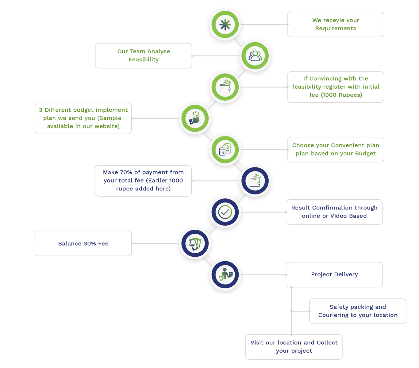
Simulation Projects Workflow

Embedded Projects Workflow