 Matlab
 Simulink
 NS3
NS3 OMNET++
 COOJA
COOJA CONTIKI OS
 NS2
NS2
Online Simulation MATLAB are laid out by us with proper Structuring and writing of your thesis here we examine some of the important procedures that are conducted by following numerous guidelines. To structure and write a thesis, we offer a well-formatted instruction, along with MATLAB code snippets, hints, and sample overviews that can help you in an effective way:
Sample Thesis Overview
- Title Page
- Abstract
- Acknowledgments
- Table of Contents
- List of Figures
- List of Tables
Chapter 1: Introduction
- Background and Purpose
- Problem Description
- Goals
- Range of the Thesis
- Arrangement of the Thesis
Chapter 2: Literature Survey
- Outline of Previous Research
- Major Discoveries from Current Studies
- Research Gaps
- Summary
Chapter 3: Methodology
- System Explanation
- Simulation Tools and Platform
- Mathematical Modeling
- Algorithm Structure
- Simulation Arrangement
Chapter 4: Implementation
- Particulars of the Simulation Code
- Explanation of Functions and Scripts
- Pseudocode for Major Algorithms
- Verification of the Model
Chapter 5: Outcomes and Discussion
- Simulation Contexts
- Analysis of Outcomes
- Comparison with Previous Project
- Discussion on Discoveries
Chapter 6: Conclusion and Upcoming Work
- Overview of Contributions
- Constraints of the Study
- Suggestions for Upcoming Research
References
Appendices
- Supplementary Data
- Collections of MATLAB Code
Sample Descriptions for Each Chapter
Chapter 1: Introduction
Background and Purpose: Regarding the research area, offer a brief summary. The reason behind the relevance of the topic has to be described.
Problem Description: The issue that we intend to solve through our project must be demonstrated in an explicit manner.
Goals: The particular goals of our exploration have to be specified.
Range of the Thesis: For our research, we need to determine the range.
Arrangement of the Thesis: The content of every section has to be explained in a concise way.
Chapter 2: Literature Survey
By considering the current studies relevant to the topic, carry out an extensive survey. The potential research gaps have to be detected, which our research intends to fulfill. Then, focus on emphasizing the major discoveries.
Chapter 3: Methodology
System Explanation: The framework or procedure that we aim to simulate has to be explained.
Simulation Tools and Platform: Appropriate for the simulation, indicate the major platform (software, hardware) and the tools (Simulink, MATLAB).
Mathematical Modeling: The mathematical models have to be depicted, which explain the framework.
Algorithm Structure: Algorithms that are utilized for simulation and enhancement should be summarized.
Simulation Arrangement: In what way the simulation is built has to be described. It is significant to encompass fixed assumptions, preliminary states, and parameters.
Chapter 4: Implementation
Regarding our MATLAB code, we have to offer elaborate explanations. Concentrate on discussing how the algorithms and models mentioned in the methodology are executed by this code.
Sample MATLAB Code Snippet:
% Example: Simulation of a simple mass-spring-damper system
% Parameters
mass = 1; % kg
spring_constant = 10; % N/m
damping_coefficient = 0.5; % Ns/m
% Time vector
t = 0:0.01:10; % 0 to 10 seconds
% Differential equation: m*x” + c*x’ + k*x = 0
% Convert to state-space form
A = [0 1; -spring_constant/mass -damping_coefficient/mass];
B = [0; 1/mass];
C = [1 0];
D = 0;
% Initial conditions
initial_conditions = [1; 0]; % Initial displacement and velocity
% Solve the system using MATLAB’s built-in solver
sys = ss(A, B, C, D);
[Y, T, X] = initial(sys, initial_conditions, t);
% Plot the results
figure;
plot(T, Y);
title(‘Mass-Spring-Damper System Response’);
xlabel(‘Time (s)’);
ylabel(‘Displacement (m)’);
grid on;
Chapter 5: Outcomes and Discussion
The outcomes of our simulations have to be depicted in a clear manner. It is crucial to involve statistical studies, tables, and graphs.
Simulation Contexts: Focus on explaining the performed experiments or various contexts.
Analysis of Outcomes: It is important to examine the significant outcomes. Then, the major discoveries have to be described.
Comparison with Previous Project: With existing projects, our outcomes must be compared.
Discussion on Discoveries: We should consider any possible constraints and the impacts of our discoveries.
Chapter 6: Conclusion and Upcoming Work
For further exploration, offer potential suggestions, and outline the major contributions. The constraints of our project have to be explained.
Overview of Contributions: The significant contributions of our study should be emphasized.
Constraints of the Study: Any constraints or problems that are faced at the time of research have to be described.
Suggestions for Upcoming Research: For upcoming work, we need to recommend potential areas that have the ability to enhance our discoveries.
References
In a reliable format, all the references have to be mentioned, which are referred to in our thesis.
Appendices
In this section, encompass all the additional materials like MATLAB Code listings, extra data, and others.
Sample MATLAB Code Listing:
% Full MATLAB code used in the thesis
function mass_spring_damper_simulation()
% Parameters
mass = 1; % kg
spring_constant = 10; % N/m
damping_coefficient = 0.5; % Ns/m
% Time vector
t = 0:0.01:10; % 0 to 10 seconds
% Differential equation: m*x” + c*x’ + k*x = 0
% Convert to state-space form
A = [0 1; -spring_constant/mass -damping_coefficient/mass];
B = [0; 1/mass];
C = [1 0];
D = 0;
% Initial conditions
initial_conditions = [1; 0]; % Initial displacement and velocity
% Solve the system using MATLAB’s built-in solver
sys = ss(A, B, C, D);
[Y, T, X] = initial(sys, initial_conditions, t);
% Plot the results
figure;
plot(T, Y);
title(‘Mass-Spring-Damper System Response’);
xlabel(‘Time (s)’);
ylabel(‘Displacement (m)’);
grid on;
end
Online Matlab Thesis writing service
MATLAB is a robust platform that is employed across numerous fields for different objectives. By encompassing concise explanations and instance of MATLAB simulation plans, we list out some interesting topics, which might be more appropriate to create your project or thesis work:
- Control Systems
- Explanation: With feedback techniques, the control frameworks have to be modeled and examined.
- Instance: For a robotic arm, a PID controller must be simulated.
% PID Controller for a robotic arm
Kp = 10;
Ki = 1;
Kd = 5;
sys = tf([Kd Kp Ki], [1 0]);
t = 0:0.01:10;
step(sys, t);
title(‘PID Controller for Robotic Arm’);
- Signal Processing
- Explanation: Through the utilization of filters and transforms, we examine and process signals.
- Instance: In order to eliminate noise from a signal, apply a low-pass filter.
% Low-pass filter
Fs = 1000; % Sampling frequency
t = 0:1/Fs:1;
x = sin(2*pi*50*t) + sin(2*pi*120*t); % Signal with two frequencies
y = lowpass(x, 100, Fs); % Low-pass filter
plot(t, x, t, y);
legend(‘Original Signal’, ‘Filtered Signal’);
title(‘Low-pass Filter’);
- Image Processing
- Explanation: For different applications, focus on handling and examining images.
- Instance: Using an image data, carry out the edge detection process.
% Edge detection
I = imread(‘peppers.png’);
I_gray = rgb2gray(I);
edges = edge(I_gray, ‘Canny’);
imshow(edges);
title(‘Edge Detection’);
- Communications
- Explanation: Concentrate on simulating interaction protocols and frameworks.
- Instance: A QPSK modulation and demodulation framework has to be simulated.
% QPSK Modulation and Demodulation
data = randi([0 1], 100, 1);
modData = pskmod(data, 4);
demodData = pskdemod(modData, 4);
scatterplot(modData);
title(‘QPSK Modulated Data’);
- Optimization
- Explanation: For better performance, we plan to enhance frameworks or parameters.
- Instance: By utilizing genetic algorithms, the model of a mechanical structure must be improved.
% Optimization using Genetic Algorithm
fun = @(x) (x(1)-2)^2 + (x(2)-3)^2;
options = optimoptions(‘ga’, ‘Display’, ‘iter’);
[x, fval] = ga(fun, 2, [], [], [], [], [], [], [], options);
disp([‘Optimal solution: ‘, num2str(x)]);
- Machine Learning
- Explanation: Specifically for forecasting and categorization, machine learning algorithms should be implemented to data.
- Instance: For digit identification, a basic neural network must be trained.
% Neural Network for Digit Recognition
load mnistdata;
net = patternnet(10);
net = train(net, xTrain, tTrain);
y = net(xTest);
perf = perform(net, tTest, y);
disp([‘Performance: ‘, num2str(perf)]);
- Power Systems
- Explanation: Electrical power grids and frameworks have to be simulated and examined.
- Instance: A basic power grid has to be simulated, which is associated with renewable energy sources.
% Simple power grid simulation
load(‘power_grid.mat’); % Load a predefined power grid model
sim(‘power_grid_model’); % Run the simulation
plot(out.tout, out.yout);
title(‘Power Grid Simulation’);
xlabel(‘Time (s)’);
ylabel(‘Voltage (V)’);
- Thermal Systems
- Explanation: We focus on examining thermal management and heat transfer frameworks.
- Instance: In a metal rod, consider the heat distribution and simulate it.
% Heat distribution in a metal rod
L = 1; % Length of the rod
T = 0:0.01:10; % Time vector
X = linspace(0, L, 50); % Space vector
alpha = 0.01; % Thermal diffusivity
u = pdepe(0, @(x,t,u,DuDx) alpha*DuDx, @(x) sin(pi*x), @(x0,u0,u1) 0, X, T);
surf(X, T, u);
title(‘Heat Distribution in a Metal Rod’);
xlabel(‘Position (m)’);
ylabel(‘Time (s)’);
zlabel(‘Temperature (C)’);
- Financial Modeling
- Explanation: Investment policies and financial markets have to be simulated.
- Instance: By employing the Black-Scholes model, stock price movement must be designed and simulated.
% Black-Scholes stock price simulation
S0 = 100; % Initial stock price
K = 100; % Strike price
r = 0.05; % Risk-free rate
sigma = 0.2; % Volatility
T = 1; % Time to maturity
[call, put] = blsprice(S0, K, r, T, sigma);
disp([‘Call option price: ‘, num2str(call)]);
disp([‘Put option price: ‘, num2str(put)]);
- Robotics
- Explanation: Robotic frameworks should be simulated, along with their control mechanisms.
- Instance: The movement of a 2-DOF robotic arm has to be simulated.
% 2-DOF robotic arm simulation
L1 = 1; L2 = 1; % Lengths of the arm segments
theta1 = pi/4; theta2 = pi/4; % Joint angles
x = L1*cos(theta1) + L2*cos(theta1 + theta2);
y = L1*sin(theta1) + L2*sin(theta1 + theta2);
plot([0 L1*cos(theta1) x], [0 L1*sin(theta1) y], ‘-o’);
xlim([-2 2]); ylim([-2 2]);
title(‘2-DOF Robotic Arm’);
xlabel(‘X’); ylabel(‘Y’);
grid on;
- Fluid Dynamics
- Explanation: Our project examines fluid dynamics by simulating fluid flow.
- Instance: With the aid of CFD, the fluid flow across an object must be simulated.
% CFD simulation of fluid flow around an object
fluidFlow = createpde(‘thermal’,’transient’);
geometryFromEdges(fluidFlow,@squareg);
thermalProperties(fluidFlow,’ThermalConductivity’,1,’MassDensity’,1,’SpecificHeat’,1);
thermalBC(fluidFlow,’Edge’,1:4,’Temperature’,0);
thermalIC(fluidFlow,0);
generateMesh(fluidFlow);
results = solve(fluidFlow,0:0.1:10);
pdeplot(fluidFlow,’XYData’,results.Temperature(:,end),’Contour’,’on’);
title(‘Fluid Flow Simulation’);
- Biological Systems
- Explanation: Biological frameworks and operations have to be designed and simulated.
- Instance: By means of the SIR model, the distribution of an infectious disease should be simulated.
% SIR model simulation
beta = 0.3; % Infection rate
gamma = 0.1; % Recovery rate
S0 = 0.99; I0 = 0.01; R0 = 0; % Initial conditions
[t, y] = ode45(@(t, y) [-beta*y(1)*y(2); beta*y(1)*y(2)-gamma*y(2); gamma*y(2)], [0 100], [S0 I0 R0]);
plot(t, y);
legend(‘Susceptible’, ‘Infected’, ‘Recovered’);
title(‘SIR Model Simulation’);
xlabel(‘Time’);
ylabel(‘Proportion’);
- Environmental Modeling
- Explanation: Concentrate on simulating ecological frameworks. Then, their implication has to be evaluated.
- Instance: In the environment, consider the distribution of pollutants and simulate it.
% Pollutant dispersion simulation
x = linspace(0, 100, 100);
y = linspace(0, 100, 100);
[X, Y] = meshgrid(x, y);
D = 0.1; % Diffusion coefficient
T = 50; % Time
C = exp(-(X.^2 + Y.^2) / (4*D*T)) / (4*pi*D*T);
surf(X, Y, C);
title(‘Pollutant Dispersion Simulation’);
xlabel(‘X’);
ylabel(‘Y’);
zlabel(‘Concentration’);
- Neural Networks
- Explanation: For different applications, we model and train neural networks.
- Instance: Particularly for handwritten digit identification, a neural network must be trained.
% Handwritten digit recognition
load(‘digits.mat’); % Load a dataset of handwritten digits
net = patternnet(10);
net = train(net, xTrain, tTrain);
y = net(xTest);
perf = perform(net, tTest, y);
disp([‘Performance: ‘, num2str(perf)]);
- Renewable Energy
- Explanation: Renewable energy frameworks have to be simulated and enhanced.
- Instance: For a specific year, consider the output of a solar panel array and simulate it.
% Solar panel array simulation
t = 0:1:365; % Days of the year
Irradiance = 1000 * sin(pi*t/365); % Simplified solar irradiance model
Efficiency = 0.15; % Solar panel efficiency
Area = 10; % Area of the solar panel array in m^2
Output = Irradiance * Efficiency * Area;
plot(t, Output);
title(‘Solar Panel Array Output’);
xlabel(‘Day’);
ylabel(‘Power Output (W)’);
- Economics
- Explanation: Various economic strategies and frameworks must be designed and simulated.
- Instance: On economic development, examine the impacts of a tax scheme and simulate it.
% Economic growth simulation
t = 0:0.1:10; % Time
GDP = exp(t); % Simplified GDP growth model
TaxRate = 0.2; % Tax rate
GDP_AfterTax = GDP * (1 – TaxRate);
plot(t, GDP, t, GDP_AfterTax);
legend(‘GDP’, ‘GDP After Tax’);
title(‘Economic Growth Simulation’);
xlabel(‘Time’);
ylabel(‘GDP’);
- Acoustics
- Explanation: Different aspects such as acoustic waves and sound propagation must be simulated.
- Instance: In a room, the distribution of sound waves has to be simulated.
% Sound wave propagation simulation
c = 343; % Speed of sound in air (m/s)
f = 1000; % Frequency of the sound wave (Hz)
t = linspace(0, 1, 1000);
x = linspace(0, 10, 100);
[X, T] = meshgrid(x, t);
P = sin(2*pi*f*(T – X/c));
surf(X, T, P);
title(‘Sound Wave Propagation’);
xlabel(‘Distance (m)’);
ylabel(‘Time (s)’);
zlabel(‘Pressure’);
- Astronomy
- Explanation: In this project, we intend to simulate celestial mechanisms and astronomical events.
- Instance: Specifically in a solar system, consider the orbits of planets and simulate it.
% Planetary orbit simulation
mu = 1; % Gravitational parameter
r0 = 1; % Initial distance
v0 = sqrt(mu/r0); % Initial velocity for a circular orbit
options = odeset(‘RelTol’, 1e-9, ‘AbsTol’, 1e-9);
[t, y] = ode45(@(t, y) [y(3); y(4); -mu*y(1)/r0^3; -mu*y(2)/r0^3], [0 10], [r0 0 0 v0], options);
plot(y(:, 1), y(:, 2));
axis equal;
title(‘Planetary Orbit Simulation’);
xlabel(‘X’);
ylabel(‘Y’);
- Materials Science
- Explanation: The activity and features of materials have to be designed and simulated.
- Instance: Stress-strain curve of a material must be simulated.
% Stress-strain curve simulation
strain = 0:0.01:0.1;
stress = 200 * strain; % Simplified linear stress-strain relationship
plot(strain, stress);
title(‘Stress-Strain Curve’);
xlabel(‘Strain’);
ylabel(‘Stress (MPa)’);
- Transportation Systems
- Explanation: Transportation frameworks and networks should be simulated and enhanced.
- Instance: Across a network of roads, examine the traffic flow and simulate it.
% Traffic flow simulation
L = 100; % Length of the road
N = 50; % Number of cars
v_max = 5; % Maximum speed
p_slow = 0.3; % Probability of slowing down
t = 0:100; % Time steps
road = zeros(L, 1); % Initialize road
cars = randperm(L, N); % Random initial positions
road(cars) = 1; % Place cars on the road
for i = t
for j = 1:N
if rand < p_slow
v = max(road(cars(j)) – 1, 0);
else
v = min(road(cars(j)) + 1, v_max);
end
next_position = mod(cars(j) + v, L) + 1;
road(cars(j)) = 0;
road(next_position) = v;
cars(j) = next_position;
end
plot(road);
title(‘Traffic Flow Simulation’);
xlabel(‘Position’);
ylabel(‘Speed’);
pause(0.1);
end
For structuring and writing a thesis, a well-formatted instruction is provided by us, encompassing some major factors. In order to build a project or thesis work, we proposed several compelling topics, along with sample MATLAB simulation plans and concise outlines.
Subscribe Our Youtube Channel
You can Watch all Subjects Matlab & Simulink latest Innovative Project Results

Our services
We want to support Uncompromise Matlab service for all your Requirements Our Reseachers and Technical team keep update the technology for all subjects ,We assure We Meet out Your Needs.
Our Services
- Matlab Research Paper Help
- Matlab assignment help
- Matlab Project Help
- Matlab Homework Help
- Simulink assignment help
- Simulink Project Help
- Simulink Homework Help
- Matlab Research Paper Help
- NS3 Research Paper Help
- Omnet++ Research Paper Help
Our Benefits
- Customised Matlab Assignments
- Global Assignment Knowledge
- Best Assignment Writers
- Certified Matlab Trainers
- Experienced Matlab Developers
- Over 400k+ Satisfied Students
- Ontime support
- Best Price Guarantee
- Plagiarism Free Work
- Correct Citations
Expert Matlab services just 1-click

Delivery Materials
Unlimited support we offer you
For better understanding purpose we provide following Materials for all Kind of Research & Assignment & Homework service.
 Programs
 Designs
 Simulations
 Results
 Graphs
 Result snapshot
 Video Tutorial
 Instructions Profile
  Sofware Install Guide
 Execution Guidance
  Explanations
 Implement Plan
Matlab Projects
Matlab projects innovators has laid our steps in all dimension related to math works.Our concern support matlab projects for more than 10 years.Many Research scholars are benefited by our matlab projects service.We are trusted institution who supplies matlab projects for many universities and colleges.
Reasons to choose Matlab Projects .org???
Our Service are widely utilized by Research centers.More than 5000+ Projects & Thesis has been provided by us to Students & Research Scholars. All current mathworks software versions are being updated by us.
Our concern has provided the required solution for all the above mention technical problems required by clients with best Customer Support.
- Novel Idea
- Ontime Delivery
- Best Prices
- Unique Work
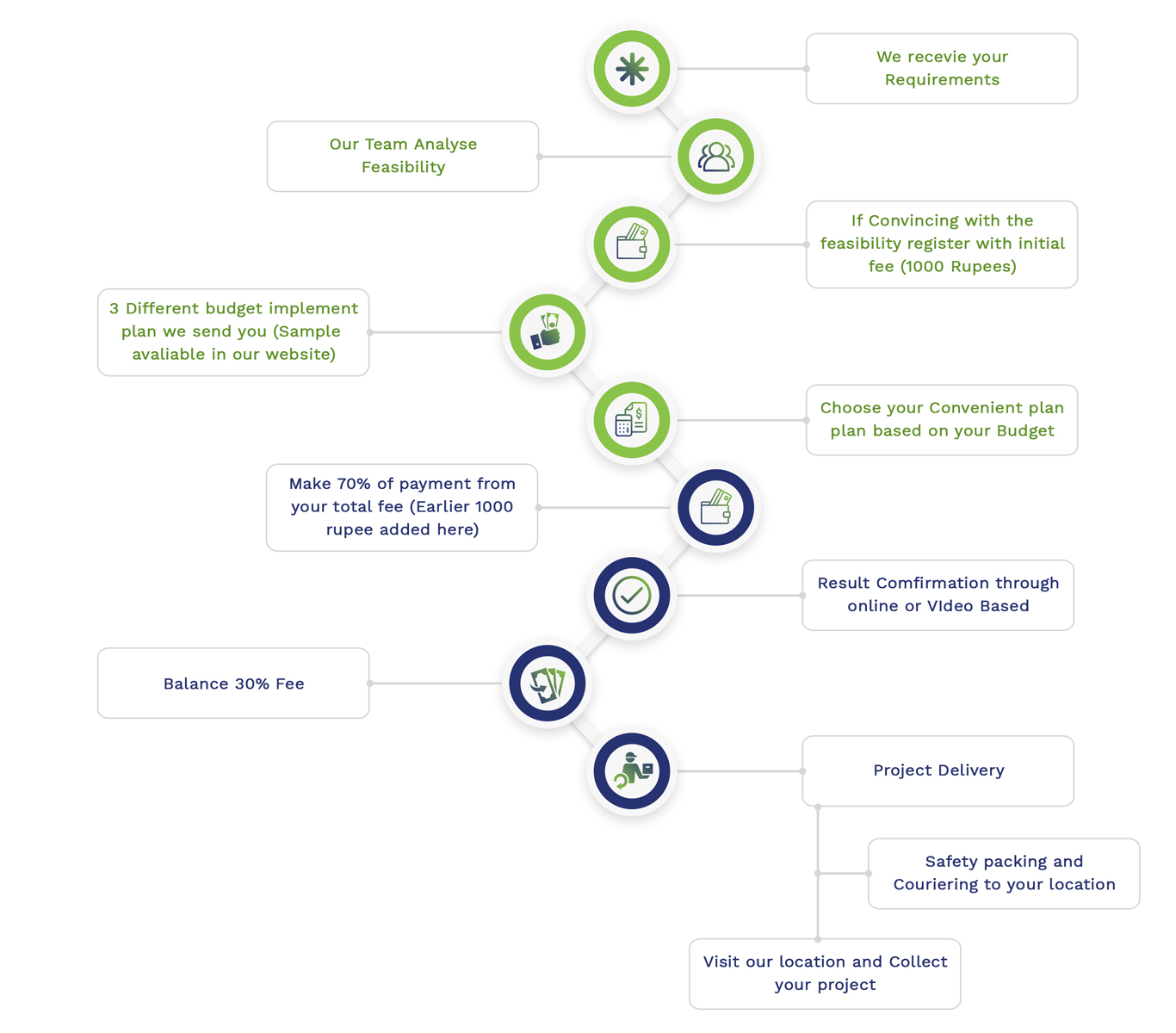
Simulation Projects Workflow
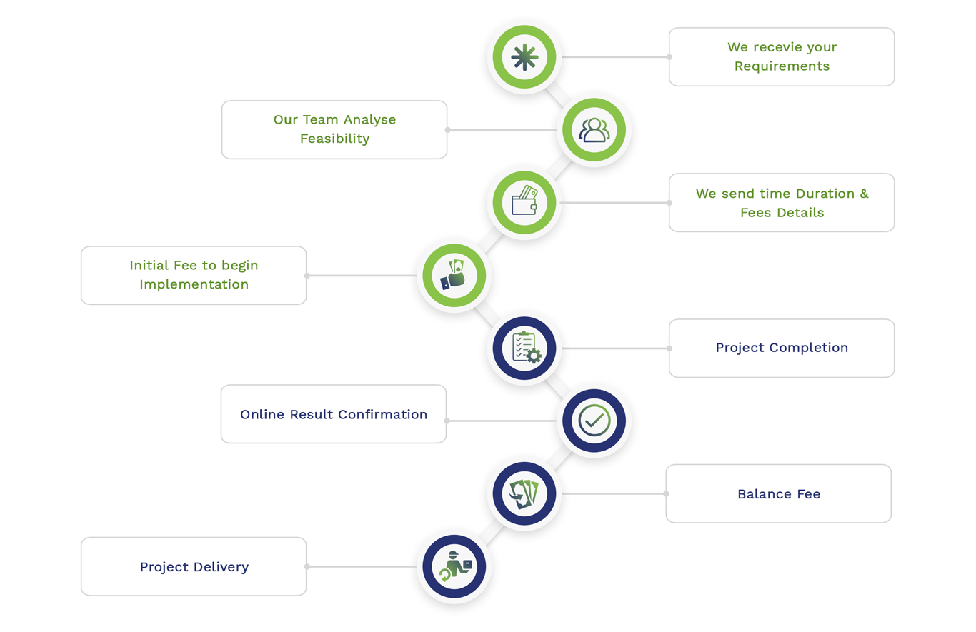
Embedded Projects Workflow